Woah! We talked about a lot of different ways of doing classification today! Let’s see what we can do about this for the Iris dataset!
Iris Dataset
Let’s load the Iris dataset! Begin by importing the load_iris tool from sklearn. This is an easy loader scheme for the iris dataset.
from sklearn.datasets import load_iris
Then, we simply execute the following to load the data.
x,y = load_iris(return_X_y=True)
We use the return_X_y argument here so that, instead of dumping a large CSV, we get the neat-cleaned input and output values.
A reminder that there is three possible flowers that we can sort by.
Decision Trees
Scikit learn has great facilities for using decision trees for classification! Let’s use some of them by fitting to the Iris dataset.
Let us begin by importing the SciKit learn tree system:
from sklearn.tree import DecisionTreeClassifier
We will fit and instantiate this classifier and fit it to the data exactly!
clf = DecisionTreeClassifier()
clf = clf.fit(x,y)
One cool thing about decision trees is that we can actually see what its doing! by looking at the series of splits and decisions. This is a function provided by tree too.
# We first import the plotting utility from matplotlib
import matplotlib.pyplot as plt
# as well as the tree plotting tool
from sklearn.tree import plot_tree

# We call the tree plot tool, which puts it on teh matplotlib graph for side effects
plot_tree(clf)
# And we save the figure
plt.savefig("tree.png")
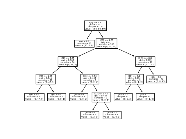
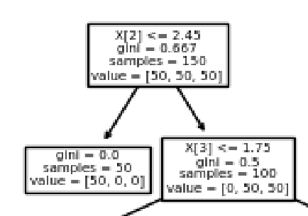
Cool! As you can see, by the end of the entire graph, the gini impurity of each node has been sorted to 0.
Apparently, if the third feature (pedal length) is smaller that 2.45, it is definitely the first type of flower!
Can you explain the rest of the divisions?
There are some arguments available in .fit of a DecisionTreeClassifier which controls for when splitting ends; for instance, max_depth controls the maximum depth by which the tree can go.
Extra Addition! Random Forests.
If you recall, we make the initial splitting decisions fairly randomly, and simply select the one with the lowest Ginni impurity. Of course, this makes the selection of the initial sets of splits very important.
What if, instead of needing to make a decision about that now, we can just deal with it later? Well, that’s where the addition of Random Forests come in.
As the name suggests, instead of having one great tree that does a “pretty good” job, we can have a lot of trees acting in ensemble! We can randomly start a bunch of random trees, and pick the selection that most would correspond with.
Random forests come from the ensemble package from sklearn; we can use it fairly simply:
from sklearn.ensemble import RandomForestClassifier
clf = RandomForestClassifier()
Wonderful! I bet you can guess what the syntax is. Instead of fitting on the whole dataset, though, we will fit on the first 145 items.
clf = clf.fit(x[:-5],y[:-5])
We can go ahead and run predict on some samples, just to see how it does on data it has not already seen before!
clf.score(x[-5:], y[-5:])
1.0
As you can see, it still does pretty well!
SVM
Let’s put another classification technique we learned today to use! Support Vector Machines. The entire syntax to manipulate support vector machines is very simple; at this point, you can probably guess it in yours sleep :)
Let’s import a SVM:
from sklearn import svm
Great. Now, we will instantiate it and fit it onto the data. SVC is the support-vector machine classifier.
clf = svm.SVC()
clf.fit(x,y)
Excellent, now, let’s score our predictions:
clf.score(x,y)
0.9733333333333334
As you can see, our data is not entirely linear! Fitting our entire dataset onto a linear SVM didn’t score perfectly, which means that the model is not complex enough to support our problem.
Scikit’s support vector machine supports lots of nonlinearity function; this is set by the argument kernel. For instance, if we wanted a nonlinear, exponential function kernel (where nonlinear function \(f(x,x’)= e^{-\gamma||\big<x,x’\big>||^2}\)), we can say:
clf = svm.SVC(kernel="rbf")
clf.fit(x,y)
clf.score(x,y)
0.9733333333333334
Looks like our results are fairly similar, though.
Naive Bayes
One last one! Its Bayes time. Let’s first take a look at how an Naive Bayes implementation can be done via Scikit learn.
One of the things that the Scikit Learn Naive Bayes estimator does differently than the one that we learned via probabilities is that it assumes that—instead of a uniform distribution (and therefore “chance of occurrence” is just occurrence divided by count), our samples are normally distributed. Therefore, we have that
\begin{equation} P(x_i | y) = \frac{1}{\sqrt{2\pi{\sigma^2}_y}}e^{\left(-\frac{(x_i-\mu_y)^2}{2{\sigma^2}_y}\right)} \end{equation}
We can instantiate such a model with the same exact syntax.
from sklearn.naive_bayes import GaussianNB
clf = GaussianNB()
clf = clf.fit(x,y)
Let’s see how it does!
clf.score(x,y)
0.96
Same thing as before, it seems simple probabilities can’t model our relationship super well. However, this is still a fairly accurate and powerful classifier.
Now you try!
- Try all three classifiers on the Wine dataset for red-white divide! Which one does better on generalizing to data you haven’t seen before?
- Explain the results of the decision trees trained on the Wine data by plotting it. Is there anything interesting that the tree used as a heuristic that came up?
- The probabilistic, uniform Naive-Bayes is fairly simple to implement write if we are using the traditional version of the Bayes theorem. Can you use Pandas to implement one yourself?