backpropegation is a special case of “backwards differentiation” to update a computation grap.h

constituents

• chain rule: suppose \(J=J\qty(g_{1}…g_{k}), g_{i} = g_{i}\qty(\theta_{1} \dots \theta_{p})\), then \(\pdv{J}{\theta_{i}} = \sum_{j=1}^{K} \pdv{J}{g_{j}} \pdv{g_{j}}{\theta_{i}}\)
• a neural network

requirements

Consider the notation in the following two layer NN:

\begin{equation} z = w^{(1)} x + b^{(1)} \end{equation}

\begin{equation} a = \text{ReLU}\qty(z) \end{equation}

\begin{equation} h_{\theta}\qty(x) = w^{(2)} a + b^{(2)} \end{equation}

\begin{equation} J = \frac{1}{2}\qty(y - h_{\theta}\qty(x))^{2} \end{equation}

1. in a forward pass, compute the values of each value \(z^{(1)}, a^{(1)}, \ldots\)
2. in a backward pass, compute…
   1. \(\pdv{J}{z^{(f)}}\): by hand
   2. \(\pdv{J}{a^{(f-1)}}\): lemma 3 below
   3. \(\pdv{J}{z^{f-1}}\): lemma 2 below
   4. \(\pdv{J}{a^{(f-2)}}\): lemma 3 below
   5. \(\pdv{J}{z^{f-2}}\): lemme 2 below
   6. and so on… until we get to the first layer
3. after obtaining all of these, we compute the weight matrices'
   1. \(\pdv{J}{W^{(f)}}\): lemma 1 below
   2. \(\pdv{J}{W^{(f-1)}}\): lemma 1 below
   3. …, until we get tot he first layer

chain rule lemmas

Pattern match your expressions against these, from the last layer to the first layer, to amortize computation.

Finally,

additional information

some issues

• Vanishing/exploding Gradients: gradient approaches 0 in saturated regime for i.e. sigmoid, resulting in them vanishing

neural networks are differentiable circuits

In a neural network, all you are allowed to do is add, subtract, multiply, divide, or elementary functions (\(\cos, \sin, \exp, \log\), activatinos etc.)

This is surprising! The usual Finite Difference Method would take \(O\qty(NL)\) (\(l\) evaluations of \(f\) each round).

Sidebar: we can compute \(\nabla^{2} f\qty(x) v\) can be computed in \(O\qty(N+l)\) by breaking it up into a matrix-vector product and applying the theorem above twice.

Motivation

• deep learning is useful by having good \(\theta\)
• we can find useful thetas by MLE
• we MLE by doing optimization to maximize the likelyhood

So we know that our loss is:

\begin{equation} J^{(j)} \qty(\theta) = \qty(y^{(i)} - h_{\theta }\qty(x^{(i)}))^{2} \end{equation}

How would we compute the gradient for \(h\qty(x)\)? where:

\begin{equation} \theta := \theta - \alpha \nabla J\qty(\theta) \end{equation}

Toy

Consider:

\begin{equation} L(a,b,c) = c(a+2b) \end{equation}

meaning, we obtain a graph that looks like:

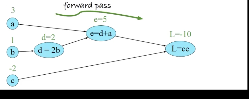
in three steps, we have:

• \(d = 2b\)
• \(e = a+d\)
• \(L = e\cdot e\)

To perform backpropagation, we compute derivatives from right to left, computing first \(\pdv{L}{L}= 1\), then, moving slowly towards the left to obtain \(\pdv{L}{c} = \pdv{L}{L}\pdv{L}{c}\), and then \(\pdv{L}{e} = \pdv{L}{L}\pdv{L}{c}\) , and then \(\pdv{L}{d} = \pdv{L}{L}\pdv{L}{e}\pdv{e}{d}\) and so forth.

Example

For one data point, let us define our neural network:

\begin{equation} h_{j} = \sigma\qty[\sum_{i}^{} x_{i} \theta_{i,j}^{(h)}] \end{equation}

\begin{equation} \hat{y} = \sigma\qty[\sum_{i}^{} h_{i}\theta_{i}^{(y)}] \end{equation}

we can define our network:

\begin{equation} L(\theta) = P(Y=y|X=x) = (\hat{y})^{y} (1-\hat{y})^{1-y} \end{equation}

from IID datasets, we can multiply the probablities together:

\begin{equation} L(\theta) = \prod_{i=1}^{n} (\hat{y_{i}})^{y_{i}} (1-\hat{y_{i}})^{1-y_{i}} \end{equation}

and, to prevent calculus and derivative instability, we take the log:

\begin{equation} LL(\theta) = \sum_{i=1}^{n}{y_{i}}\log (\hat{y_{i}}) \cdot ( 1-y_{i} )\log (1-\hat{y_{i}}) \end{equation}

We want to maximise this, meaning we perform gradient ascent on this statement. Recall the chain rule; so we can break each layer down:

\begin{equation} \pdv{LL(\theta)}{\theta_{ij}^{h}} = \pdv{LL(\theta)}{\hat{y}} \pdv{\hat{y}}{h_{j}} \pdv{h_{j}}{\theta_{ij}^{h}} \end{equation}

furthermore, for any summation,

\begin{equation} \dv x \sum_{i=0}^{} x = \sum_{i=0}^{}\dv x x \end{equation}

So we can consider our derivatives with respect to each data point. When going about the second part, recall an important trick:

\begin{equation} \pdv{h_{i}} \qty[\sum_{i}^{} h_{i}\theta_{i}^{(y)}] \end{equation}

you will note that, for the inside derivative, much the summation expands

Example2

Consider the following two layer NN:

\begin{equation} z = w^{(1)} x + b^{(1)} \end{equation}

\begin{equation} a = \text{ReLU}\qty(z) \end{equation}

\begin{equation} h_{\theta}\qty(x) = w^{(2)} a + b^{(2)} \end{equation}

\begin{equation} J = \frac{1}{2}\qty(y - h_{\theta}\qty(x))^{2} \end{equation}

Notice now by the chain rule (and some careful index tracking) we have:

\begin{equation} \pdv{J}{W^{[1]}} = \pdv{J}{z} \pdv{z}{w^{(1)}} = \pdv{J}{z} x^{T} \end{equation}

\begin{equation} \pdv{J}{b^{(1)}} = \pdv{J}{z} 1 = \pdv{J}{z} \end{equation}

\begin{equation} \pdv{J}{z} = \pdv{J}{a} \odot \text{ReLU}’ \qty(z) \end{equation}

\begin{equation} f\qty(x) = g\qty(x) + y \end{equation}

\begin{equation} g\qty(x) = h\qty(x) + z \end{equation}

\begin{equation} h\qty(x) = x \end{equation}

\begin{equation} \pdv{f}{x} = \pdv{f}{g} \pdv{g}{h} \pdv{h}{x} \end{equation}