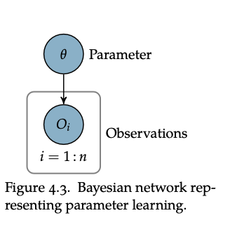
We treat this as an inference problem in Naive Bayes: observations are independent from each other.
Instead of trying to compute a \(\theta\) that works for Maximum Likelihood Parameter Learning, what we instead do is try to understand what \(\theta\) can be in terms of a distribution.
That is, we want to get some:
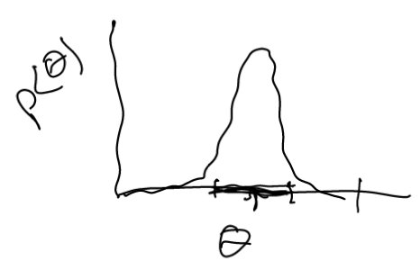
“for each value of \(\theta\), what’s the chance that that is the actual value”
To do this, we desire:
\begin{equation} p(\theta | D) \end{equation}
“what’s the probability of theta being at a certain value given the observations we had.”
And to obtain the actual the actual value, we calculate the expectation of this distribution:
\begin{equation} \hat{\theta} = \mathbb{E}[\theta] = \int \theta p(\theta | D) \dd{\theta} \end{equation}
If its not possible to obtain such an expected value, we then calculate just the mode of the distribution (like where the peak probability of \(\theta\) is) by:
\begin{equation} \hat{\theta} = \arg\max_{\theta} p(\theta | D) \end{equation}
Bayesian Parameter Learning on Binary Distributions
We are working in a Naive Bayes environment, where we assume that \(o_{1:m}\) are conditionally independent. Then, we essentially consider each class as carrying some parameter \(\theta\) which contains the possibility of that class happening.
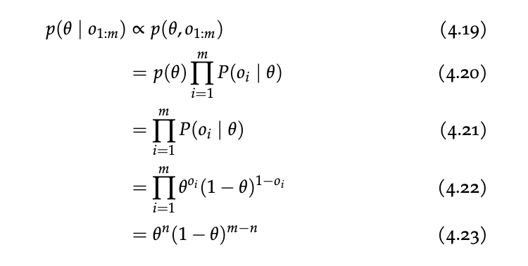
Using the same steps as inference with Naive Bayes and some algebra:
\begin{equation} p(\theta | o_{1:m}) \propto p(\theta, o_{1:m}) \end{equation}
Now, we would like to normalize this function for \(\theta \in [0,1]\), so, we get:
\begin{equation} \int_{0}^{1} \theta^{n}(1-\theta)^{m-n}\dd{\theta} = \frac{\Gamma(n+1) \Gamma(m-n+1)}{\Gamma(m+2)} \end{equation}
where, \(\Gamma\) is a real valued factorial generalization, and this entire integral is often called the “Beta Function”
Normalizing the output, we have that:
\begin{align} p(\theta | o_{1:m}) &\propto p(\theta, o_{1:m}) \\ &= \frac{\Gamma(m+2)}{\Gamma(n+1) \Gamma(m-n+1)} \theta^{n} (1-\theta)^{m-n} \\ &= Beta(\theta | n+1, m-n +1) \end{align}
where \(m\) is the sample size and \(n\) is the number of events in the sample space.
Beta Distribution
Suppose you had a non-uniform prior:
- Prior: \(Beta(\alpha, \beta)\)
- Observe: \(m_1\) positive outcomes, \(m_2\) negative outcomes
- Posterior: \(Beta(\alpha+m_1, \beta+m_2)\)
That is: for binary outcomes, the beta distribution can be updated without doing any math.
For instance, say we had:
\begin{equation} \theta_{t} = Beta(\alpha, \beta) \end{equation}
and we observed that \(o_{i} = 1\), then:
\begin{equation} \theta_{t+1} = Beta(\alpha+1, \beta) \end{equation}
instead, if we observed that \(o_{i} = 0\), then:
\begin{equation} \theta_{t+1} = Beta(\alpha, \beta+1) \end{equation}
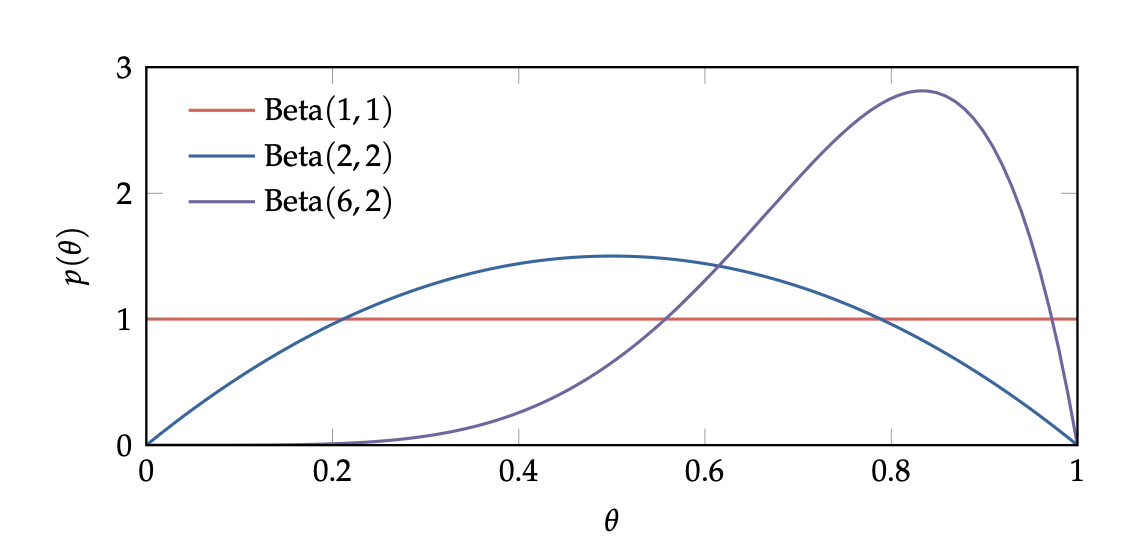
Essentially: MAGNITUDE of beta distribution governs how small the spread is (higher magnitude smaller spread), and the balance between the two values represents how much skew there is.
Beta is a special distribution which takes parameters \(\alpha, \beta\),and has mean:
\begin{equation} \frac{\alpha}{\alpha + \beta} \end{equation}
and variance:
\begin{equation} \frac{ab}{(a+b)^{2}(a+b+1)} \end{equation}
and has mode:
\begin{equation} \frac{\alpha -1 }{\alpha + \beta -2} \end{equation}
when \(\alpha > 1\) and \(\beta > 1\).
This means that, at \(beta(1,1)\), we have a inform distribution
Laplace Smoothing
Laplace Smoothing is a prior where:
\begin{equation} prior\ X \sim Beta(2,2) \end{equation}
so you just add \(2\) to each of our output pseudo counts.
see also Laplace prior, where you use Laplace Smoothing for your prior
Total Probability in beta distributions
Recall, for total probability, beta is a special distribution which takes parameters \(\alpha, \beta\),and has expectation:
\begin{equation} \frac{\alpha}{\alpha + \beta} \end{equation}
and has mode:
\begin{equation} \frac{\alpha -1 }{\alpha + \beta -2} \end{equation}
Choosing a prior
- do it with only the problem and no knowledge of the data
- uniform typically works well, but if you have any reason why it won’t be uniform (say coin flip), you should count accordingly such as making the distribution more normal with \(Beta(1,1)\)
Dirichlet Distribution
We can generalize the Bayesian Parameter Learning on Binary Distributions with the Dirichlet Distribution.
For \(n\) parameters \(\theta_{1:n}\) (\(n-1\) of which independent, because we know that \(\sum \theta_{i} = 1\)), where \(\theta_{j}\) is the probability that the \(j\) th case of the categorical distribution happening.
Now:
\begin{equation} Dir(\theta_{1:n} | \alpha) = \frac{\Gamma(\alpha_{0})}{\prod_{i=1}^{n} \Gamma(\alpha_{i})} \prod_{i=1}^{n} \theta_{i}^{\alpha_{i}-1} \end{equation}
whereby:
\begin{equation} \alpha_{j} = prior + count \end{equation}
for \(j \geq 1\), and
\begin{equation} \alpha_{0} = prior + total_{}count \end{equation}
whereby prior is your initial distribution. If its uniform, then all prior equals one.
The expectation for each \(\theta_{i}\) happening is:
\begin{equation} \mathbb{E}[\theta_{i}] = \frac{a_{i}}{\sum_{j=1}^{n} \alpha_{j}} \end{equation}
and, with \(a_{i} > 1\), the $i$th mode is:
\begin{equation} \frac{a_{i}-1 }{\sum_{j=1}^{n} a_{j}-n} \end{equation}
expectation of a distribution
For Beta Distribution and Dirichlet Distribution, the expectation of their distribution is simply their mean.
if you say want to know what the probability of \(P(thing|D)\), you can integrate over all \(P(thing|\theta)\):
\begin{equation} \int^{1}_{0} P(thing|\theta)P(\theta)d\theta \end{equation}
The first thing is just the actual value of \(\theta\) (because \(\theta\) is literally the probability of \(thing\) happening). The second thing is the probability of that \(\theta\) actually happening.
This, of course, just add up to the expected value of \(\theta\), which is given above:
\begin{equation} \frac{\alpha}{\alpha + \beta} \end{equation}