Brownian Motion

Brownian Motion is the pattern for measuring the convergence of random walk through continuous timing.

discrete random walk

discrete random walk is a tool used to construct Brownian Motion. It is a random walk which only takes on two discrete values at any given time: $\Delta$ and its additive inverse $-\Delta$. These two cases take place at probabilities $\pi$ and $1-\pi$.

Therefore, the expected return over each time $k$ is:

\begin{equation} \epsilon_{k} = \begin{cases} \Delta, p(\pi) \\ -\Delta, p(1-\pi) \end{cases} \end{equation}

(that, at any given time, the expectation of return is either—with probability $π$—$\Delta$, or–with probability $1-π$—$-\Delta$.

This makes $\epsilon_{k}$ independently and identically distributed. The price, then, is formed by:

\begin{equation} p_{k} = p_{k-1}+\epsilon_{k} \end{equation}

and therefore the price follows a random walk.

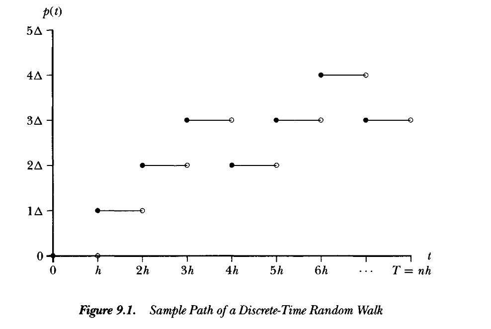
Such a discrete random walk can look like this:

We can split this time from $[0,T]$ into $n$ pieces; making each segment with length $h=\frac{T}{n}$. Then, we can parcel out:

\begin{equation} p_{n}(t) = p_{[\frac{t}{h}]} = p_{[\frac{nt}{T}]} \end{equation}

Descretized at integer intervals.

At this current, discrete moments have expected value $E[p_{n}(T)] = n(\pi -(1-\pi))\Delta$ and variance $Var[p_{n}(T)]=4n\pi (1-\pi)\Delta^{2}$. #why

Now, if we want to have a continuous version of the descretized interval above, we will maintain the finiteness of $p_{n}(T)$ but take $n$ to $\infty$. To get a continuous random walk needed for Brownian Motion, we adjust $\Delta$, $\pi$, and $1-\pi$ such that the expected value and variance tends towards the normal (as we expect for a random walk); that is, we hope to see that:

\begin{equation} \begin{cases} n(\pi -(1-\pi))\Delta \to \mu T \\ 4n\pi (1-\pi )\Delta ^{2} \to \sigma^{2} T \end{cases} \end{equation}

To solve for these desired convergences into the normal, we have probabilities $\pi, (1-\pi), \Delta$ such that:

\begin{equation} \begin{cases} \pi = \frac{1}{2}\qty(1+\frac{\mu \sqrt{h}}{\sigma})\\ (1-\pi) = \frac{1}{2}\qty(1-\frac{\mu \sqrt{h}}{\sigma})\\ \Delta = \sigma \sqrt{h} \end{cases} \end{equation}

where, $h = \frac{1}{n}$.

So looking at the expression for $\Delta$, we can see that as $n$ in increases, $h =\frac{1}{n}$ decreases and therefore $\Delta$ decreases. In fact, we can see that the change in all three variables track the change in the rate of $\sqrt{h}$; namely, they vary with O(h).

\begin{equation} \pi = (1-\pi) = \frac{1}{2}+\frac{\mu \sqrt{h}}{2\sigma} = \frac{1}{2}+O\qty(\sqrt{h}) \end{equation}

Of course:

\begin{equation} \Delta = O\qty(\sqrt{h}) \end{equation}

So, finally, we have the conclusion that:

as $n$ (number of subdivision pieces of the time domain $T$) increases, $\frac{1}{n}$ decreases, $O\qty(\sqrt{h})$ decreases with the same proportion. Therefore, as $\lim_{n \to \infty}$ in the continuous-time case, the probability of either positive or negative delta ($\pi$ and $-\pi$ trends towards each to $\frac{1}{2}$)
by the same vein, as $\lim_{n \to \infty}$, $\Delta \to 0$

Therefore, this is a cool result: in a continuous-time case of a discrete random walk, the returns (NOT! just the expect value, but literal $\Delta$) trend towards $+0$ and $-0$ each with $\frac{1}{2}$ probability.

actual Brownian motion

Given the final results above for the limits of discrete random walk, we can see that the price moment traced from the returns (i.e. $p_{k} = p_{k-1}+\epsilon_{k}$) have the properties of normality ($p_{n}(T) \to \mathcal{N}(\mu T, \sigma^{2}T)$)

True Brownian Motion follows, therefore, three basic properties:

$B_{t}$ is normally distributed by a mean of $0$, and variance of $t$
For some $s<t$, $B_{t}-B_{s}$ is normally distributed by a mean of $0$, and variance of $t-s$
Distributions $B_{j}$ and $B_{t}-B_{s}$ is independent

Standard Brownian Motion

Brownian motion that starts at $B_0=0$ is called Standard Brownian Motion

quadratic variation

The quadratic variation of a sequence of values is the expression that:

\begin{equation} \sum_{i=0}^{N-1} (x_{i+1}-x_i)^{2} \end{equation}

On any sequence of values $x_0=0,\dots,x_{N}=1$ (with defined bounds), the quadratic variation becomes bounded.