We aim to solve for a fixed-sized controller based policy using gradient ascent. This is the unconstrained variation on PGA.
Recall that we seek to optimize, for some initial node \(x^{(1)}\) and belief-state \(b\), we want to find the distribution of actions and transitions \(\Psi\) and \(\eta\), which maximizes the utility we can obtain based on initial state:
\begin{equation} \sum_{s}b(s) U(x^{(1)}, s) \end{equation}
Recall that \(U(x,s)\) is given by:
\begin{equation} U(x, s) = \sum_{a}^{} \Psi(a|x) \qty[R(s,a) + \gamma \qty(\sum_{s’}^{} T(s’|s,a) \sum_{o}^{} O(o|a, s’) \sum_{x’}^{} \eta(x’|x,a,o) U(x’, s’)) ] \end{equation}
where
- \(X\): a set of nodes (hidden, internal states)
- \(\Psi(a|x)\): probability of taking an action
- \(\eta(x’|x,a,o)\) : transition probability between hidden states
Let’s first develop some tools which can help us linearize the objective equation given above.
We can define a transition map (matrix) between any two controller-states (latent + state) as:
\begin{equation} T_{\theta}((x,s), (x’,s’)) = \sum_{a} \Psi(a | x) T(s’|s,a) \sum_{o} O (o|a,s’) \eta (x’|x,a,o) \end{equation}
where \(\bold{T}_{\theta} \in \mathbb{R}^{|X \times S| \times |X \times S|}\) .
Further, we can parameterize reward over \(R(s,a)\) for:
\begin{equation} R_{\theta}((x, s)) = \sum_{a} \Psi(a|x) R(s,a) \end{equation}
where \(R_{\theta}\in \mathbb{R}^{|X \times S|}\)
(i.e. the reward of being in each controller state is the expected reward over all possible actions at that controller state).
And now, recall the procedure for Bellman Expectation Equation; having formulated the transition and reward at any given controller state \(X \times S\), we can write:
\begin{equation} \bold{u}_{\theta} = \bold{r}_{\theta} + \gamma \bold{T_{\theta}}\bold{u}_{\theta} \end{equation}
note that this vector \(\bold{U} \in \mathbb{R}^{|X \times S}}\). Therefore, to write out an “utility of belief” (prev. \(b^{\top} U\) where \(U \in \alpha\) some alpha vector over states), we have to redefine a:
\begin{equation} \bold{\beta}_{xs}, \text{where} \begin{cases} \bold{\beta}_{xs} = b(s), if\ x = x^{(1)} \\ 0 \end{cases} \end{equation}
Finally, then we can rewrite the objective as:
\begin{equation} \beta^{\top} \bold{U}_{\theta} \end{equation}
where we seek to use gradient ascend to maximize \(\bold{U}_{\theta}\).
Writing this out, we have:
\begin{equation} \bold{u}_{\theta} = \bold{r}_{\theta} + \gamma \bold{T}_{\theta} \bold{u}_{\theta} \end{equation}
which gives:
\begin{equation} \bold{u}_{\theta} = (\bold{I} - \gamma \bold{T}_{\theta})^{-1} \bold{r}_{\theta} \end{equation}
Let’s call \(\bold{Z} = (\bold{I}-\gamma \bold{T}_{\theta})\), meaning:
\begin{equation} \bold{u}_{\theta} = \bold{Z}^{-1} \bold{r}_{\theta} \end{equation}
Finally, to gradient ascent, we better get the gradient. So… its CHAIN RULE TIME
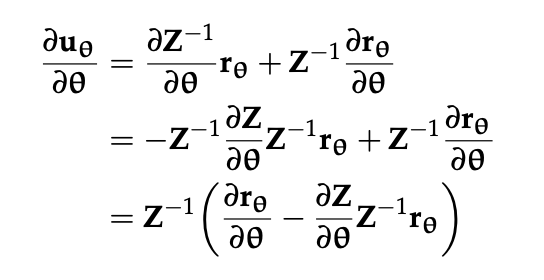
Recall that \(\theta\) at this point refers to both \(\eta\) and \(\Psi\), so we need to take a partial against each of those variables. After doing copious calculus in Alg4DM pp 485, we arrive at the update expressions.