Let’s consider greedy Decision Tree learning.
greedy procedure
- initial tree—no split: always predict the majority class \(\hat{y} = \text{maj}\qty(y), \forall x\)
- for each feature \(h\qty(x)\)
- split data according to feature
- compute classification error of the split
- choose \(h^{*}\qty(x)\) with the lowest error after splitting
- loop until stop
stopping criteria
- each node agrees on \(y\) (the tree fits data exactly)
- exhausted on all features (nothing to split on)
additional information
threshold splitting
We are going to perform what’s called a “threshold split.” Choose thresholds between two points as the “split values” to check. Now, how do we deal with splitting twice? We can until we get bored or we over fit.
dealing with overfitting
early stopping
Stop the tree before it becomes too complex.
limiting tree depth (choose max_depth at the point where val error begins to increase)
- we may also want some branches to go deeper than others
- however, this could exacerbate non-greedy problems
don’t consider splits that don’t cause a sufficient error decrease
don’t split on leafs with too few data points
pruning
We want to regularize the tree (i.e. balancing measure of fit — accuracy, measure of complexity — complexity.)
\begin{equation} C\qty(T) = \text{Error}\qty(T) + \lambda L\qty(T) \end{equation}
where \(C\) is the cost, \(T\) is the tree, \(\text{Error}\) is the normal error parameter, \(L\) is the number of leafs. Using this measure, we can prune the tree:
- start bottom-up (i.e. look at the leafs)
- get rid of subtrees at a time, increasing order in size of the subtree you threw away (i.e. depth from bottom), measure if doing a particular node would lower the cost
decision trees vs logistic regression
- decision tree splits dataset via hyper-rectangles (i.e. a line that is a single variable with no dependence, x>n, x=n, etc., lines)
- logistic regression splits data via hype-planes (i.e. a line that’s a function of other variables)
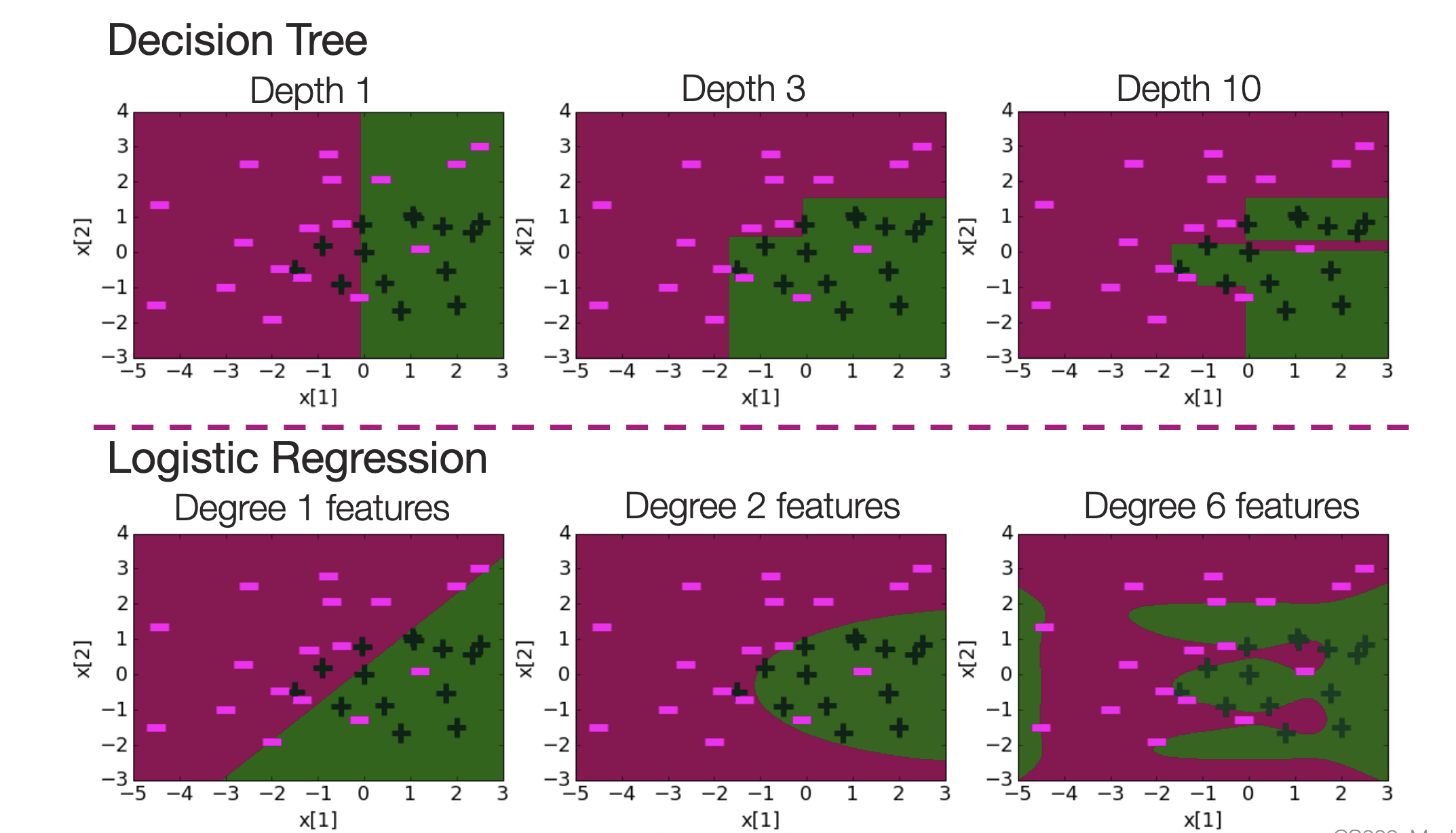
(image from Carlos Guestrin’s slides)
why don’t we stop splitting when all features lead to the same loss
consider XOR:
| x | y | XOR |
|---|---|---|
| 0 | 0 | 0 |
| 0 | 1 | 1 |
| 1 | 0 | 1 |
| 1 | 1 | 0 |
Notice splitting on either x or y will give you nothing, but you have to split on one of them, and then another, to get to \(100\%\) accuracy. i.e. splits may set you up for performance in future splits.
the greedy procedure can be arbitrarily bad
Consider XOR with feature x1 and x2; then, add features x3 …. xn each of which alone (independently) reduces error by \(\epsilon\). Splitting on x1 and x2 alone wouldn’t give you any gain (i.e. you need 2 steps), but then you will be splitting on a humongous number of barely useful features because they give you one step information.
motivation
Suppose you are interested in predicting loan defaults. Consider we taking information \(x_{i}\) from a user (defaults, credit scores, etc.), and builds a boolean classifier for whether or not the sample will default \(y_{i}\).
The learning problem: given \(N\) training samples \(\qty(x^{(i)}, y^{(i)})\), we want to predict the accuracy of the system: number of incorrect predictions divided by total number of samples.
optimality: the smallest possible tree that memorizes the data. This is NP hard (since exponentially number of trees).
gini impurity
Its usually presented in terms of Gini impurity in a multi-class setting; as in the “score” is formalized as “Gini Purity”:
\begin{equation} G_{f} = \sum_{j=1}^{N} p_{f}(j) \cdot p_{f}(\neg j) \end{equation}
with \(N\) classes and \(f \in F\) features, and where \(p_{f}(j)\) means the probability that, for the subset of the data with condition \(f\), a random sample takes on class \(j\). Then, we select the feature:
\begin{equation} f_{split} = \arg\min_{f}\qty( G_{f} + G_{\neg f}) \end{equation}
We want this because we want each feature split to be “pure”—we want there to be either high probability of each split containing one class, or absolutely not containing it, so either \(p_{f}(j)\) or \(p_{f}(\neg j)\) should be very low.
Yet, this textbook uses a goofy representation where their splitting score is, after splitting by some feature \(f\) the count in each group having the majority class of that group—which functionally measures the same thing (class “purity” of each group); ideally, we want this value to be high, so we take argmax of it.
also I’m pretty sure we can recycle features instead of popping them out; check me on this.