deep learning is MLE performed with neural networks. A neural network is many logistic regression pieces (sic.?) stack on top of each other.
We begin motivating this with trying to solve MNIST with logistic regression. What a time to be alive. After each layer of deep learning, we are going to use a layer of “hidden variable”, made of singular logistic regressions,
Notation:
\(x\) is the input, \(h\) is the hidden layers, and \(\hat{y}\) is the prediction.
We call each weight, at each layer, from \(x_{i}\) to \(h_{j}\), \(\theta_{i,j}^{(h)}\). At every neuron on each layer, we calculate:
\begin{equation} h_{j} = \sigma\qty[\sum_{i}^{} x_{i} \theta_{i,j}^{(h)}] \end{equation}
\begin{equation} \hat{y} = \sigma\qty[\sum_{i}^{} h_{i}\theta_{i}^{(y)}] \end{equation}
note! we often
backpropegation
backpropegation is a special case of “backwards differentiation” to update a computation grap.h
Toy
Consider:
\begin{equation} L(a,b,c) = c(a+2b) \end{equation}
meaning, we obtain a graph that looks like:
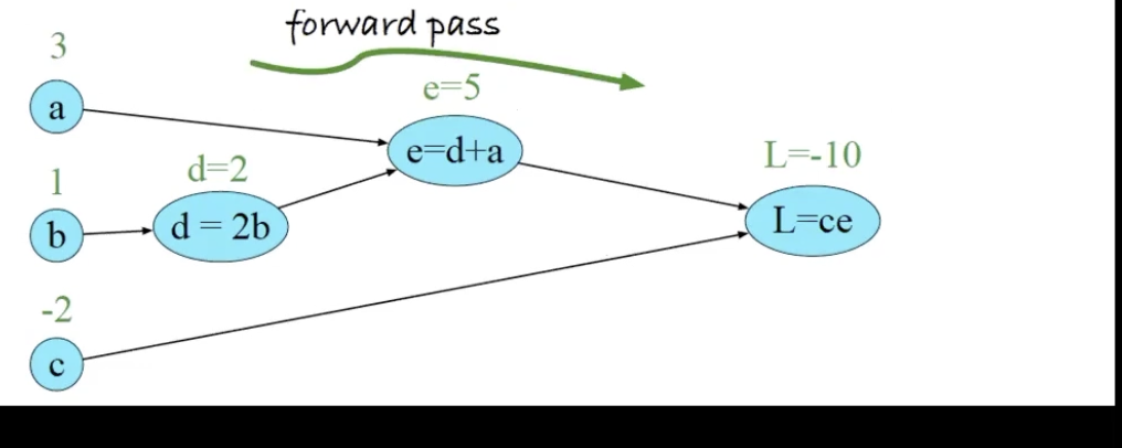
in three steps, we have:
- \(d = 2b\)
- \(e = a+d\)
- \(L = e\cdot e\)
To perform backpropagation, we compute derivatives from right to left, computing first \(\pdv{L}{L}= 1\), then, moving slowly towards the left to obtain \(\pdv{L}{c} = \pdv{L}{L}\pdv{L}{c}\), and then \(\pdv{L}{e} = \pdv{L}{L}\pdv{L}{c}\) , and then \(\pdv{L}{d} = \pdv{L}{L}\pdv{L}{e}\pdv{e}{d}\) and so forth.
Motivation
- deep learning is useful by having good \(\theta\)
- we can find useful thetas by MLE
- we MLE by doing optimization to maximize the likelyhood
Example
For one data point, let us define our neural network:
\begin{equation} h_{j} = \sigma\qty[\sum_{i}^{} x_{i} \theta_{i,j}^{(h)}] \end{equation}
\begin{equation} \hat{y} = \sigma\qty[\sum_{i}^{} h_{i}\theta_{i}^{(y)}] \end{equation}
we can define our network:
\begin{equation} L(\theta) = P(Y=y|X=x) = (\hat{y})^{y} (1-\hat{y})^{1-y} \end{equation}
from IID datasets, we can multiply the probablities together:
\begin{equation} L(\theta) = \prod_{i=1}^{n} (\hat{y_{i}})^{y_{i}} (1-\hat{y_{i}})^{1-y_{i}} \end{equation}
and, to prevent calculus and derivative instability, we take the log:
\begin{equation} LL(\theta) = \sum_{i=1}^{n}{y_{i}}\log (\hat{y_{i}}) \cdot ( 1-y_{i} )\log (1-\hat{y_{i}}) \end{equation}
We want to maximise this, meaning we perform gradient ascent on this statement. Recall the chain rule; so we can break each layer down:
\begin{equation} \pdv{LL(\theta)}{\theta_{ij}^{h}} = \pdv{LL(\theta)}{\hat{y}} \pdv{\hat{y}}{h_{j}} \pdv{h_{j}}{\theta_{ij}^{h}} \end{equation}
furthermore, for any summation,
\begin{equation} \dv x \sum_{i=0}^{} x = \sum_{i=0}^{}\dv x x \end{equation}
So we can consider our derivatives with respect to each data point. When going about the second part, recall an important trick:
\begin{equation} \pdv{h_{i}} \qty[\sum_{i}^{} h_{i}\theta_{i}^{(y)}] \end{equation}
you will note that, for the inside derivative, much the summation expands