Divide by \(2\pi\), or, how I learned to start worrying and hate Fourier Transforms.
Hello all. Good news first: our frequency theory is now correctly validated by data.
If you want a band-aid for the answer, here it is: divide everything we get out of the cantilever equations by \(2\pi\); then, use the correct linear mass density: our Google sheets was off by a factor of almost \(4\) because of later-corrected apparent measurement error.
The bad news? You get pages of algebra to justify how, while getting a whole run-down of our entire theory so far for kicks.
Our story begins at what popped out of the other end of the Euler-Lagrange equations (if you want the start of the Lagrangian analysis, read this from Mark, and plug the resulting Lagrangian into the Euler-Lagrange equation of the right shape.) But, either way, out will pop this fourth-order partial differential equation:
\begin{equation} EI\pdv[4]{w}{x} = -\mu \pdv[2]{w}{t} \end{equation}
where, \(w(x,t)\) is a function of displacement by location by time, \(E\) the elastic modulus, and \(I\) the second moment of bending area.
Now, fourth-order diffequs are already pain. PARTIAL forth order diffequs sounds darn near impossible. Wikipedia, to their credit, helpfully suggests the following to help tackle this problem:
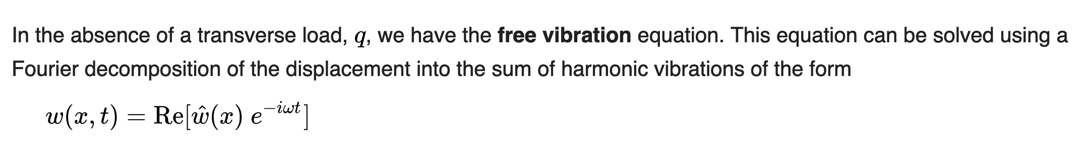
You see, as we are trying to isolate possible individual frequencies, it make sense to essentially run a Fourier Transform on our algebra, to get the possible amplitude at each frequency \(\hat{w}(x)\), given some frequency \(\omega\) (no idea why they use \(\omega\), I will use \(f\) for the rest of this article.)
To perform this analysis, Wikipedia suggests that we substitute our \(w(x,t)\) with its Fourier Definition, which is written as a function of the Fourier-decomposed version of the function \(\hat{w}(x)\) (real component only, as imaginary pairs serve only as the conjugate), and then re-isolate those decomposed \(\hat{w}(x)\). In this way, we get rid of the time dimension as sine waves oscillate ad infinium. Makes total sense.
EXCEPT WHAT WIKIPEDIA GAVE ABOVE TO SUBSTITUTE IN ISN’T THE CORRECT FOURIER DECOMPOSITION
Here’s the actual Fourier Transform intergral:
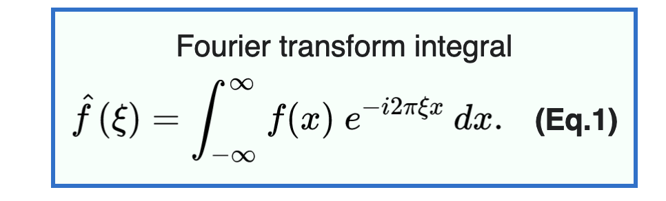
where, \(\zeta=\omega=f\) , \(f(x) = \hat{w}(x)\).
WHAT DO YOU NOTICE? AN EXTRA \(2\pi\).
THIS ALSO MEANS THAT THE FREQUENCY ANALYSTS IN THE REST OF THAT WIKI ARTICLE IS WRONG
Ok. I collect myself.
So, we now have that:
\begin{equation} w(x,t) = Re\qty[\hat{w}(x)e^{-i 2\pi ft}] \end{equation}
Recall that we are trying to substitute this into
\begin{equation} EI\pdv[4]{w}{x} = -\mu \pdv[2]{w}{t} \end{equation}
Taking two derivatives of the above Fourier decomposition equation by time (which is the dimension we are trying to get rid of to make the diffequ not partial), we have:
\begin{align} \pdv[2]{w(x,t)}{t} &= \pdv[2] t Re\qty[\hat{w}(x)e^{-i2\pi ft}] \\ &= Re\qty[\hat{w}(x)\pdv[2] t e^{-i2\pi ft}] \\ &= Re\qty[\hat{w}(x)(2\pi f)^{2} \cdot e^{-i2\pi ft}\dots] \end{align}
Now, given we are only dealing with the real components of these things, everything on the \(e^{-i\dots }\) part of the function wooshes away, cleanly leaving us with:
\begin{equation} \pdv[2]{w(x,t)}{t} &= \hat{w}(x)(2\pi f)^{2} \end{equation}
Yay! No longer differential. Substituting that into our original expression, and making the partials not partial anymore:
\begin{equation} EI\pdv[4]{w}{x} + \mu \hat{w}(x)(2\pi f)^{2}= 0 \end{equation}
Excellent. Now, onto solving this. The basic way to solve this is essentially to split the fourth-order differential into a 4x4 matrix, each one taking another derivative of the past. Then, to get a characteristic solution, you take its eigenvalues.
But instead of going about doing that, I’m going to give up and ask a computer. In the code, I am going to substitute \(p\) for \(2\pi\) temporarily because FriCAS gets a little to eager to convert things into their sinusoidal forms if we leave it as \(2\pi\).
E,I,u,f = var("E I u f")
x, L = var("x L")
w = function('w')(x)
p = var("p")
_c0, _c1, _c2, _c3 = var("_C0 _C1 _C2 _C3")
fourier_cantileaver = (E*I*diff(w, x, 4) - u*(p*f)^2*w == 0)
fourier_cantileaver
-f^2*p^2*u*w(x) + E*I*diff(w(x), x, x, x, x) == 0
solution = desolve(fourier_cantileaver, w, ivar=x, algorithm="fricas").expand()
latex(solution)
\begin{equation} \hat{w}(x) = _{C_{1}} e^{\left(\sqrt{f} \sqrt{2\pi} x \left(\frac{u}{E I}\right)^{\frac{1}{4}}\right)} + _{C_{0}} e^{\left(i \, \sqrt{f} \sqrt{2\pi} x \left(\frac{u}{E I}\right)^{\frac{1}{4}}\right)} + _{C_{2}} e^{\left(-i \, \sqrt{f} \sqrt{2\pi} x \left(\frac{u}{E I}\right)^{\frac{1}{4}}\right)} + _{C_{3}} e^{\left(-\sqrt{f} \sqrt{2 \pi} x \left(\frac{u}{E I}\right)^{\frac{1}{4}}\right)} \end{equation}
Ok, so we have that each component solution is a combination of a bunch of stuff, times \(\pm i\) or \(\pm 1\). We are going to declare everything that’s invariant in the exponent to be named \(\beta\):
\begin{equation} \beta := \sqrt{2\pi f} \qty(\frac{u}{EI})^{\frac{1}{4}} \end{equation}
And given this, we can then write the general solution for displacement by location (\(w\)) determined above more cleanly as:
\begin{equation} \hat{w}(x) = _{C_{1}} e^{\beta x} + _{C_{0}} e^{ \beta ix} + _{C_{2}} e^{-\beta ix} + _{C_{3}} e^{-\beta x} \end{equation}
We will make one more substitution—try to get the \(e^{x}\) into sinusoidal form. We know this is supposed to oscillate, and it being in sinusoidal makes the process of solving for periodic solutions easier.
Recall that:
\begin{equation} \begin{cases} \cosh x = \frac{e^{x}+e^{-x}}{2} \\ \cos x = \frac{e^{ix}+e^{-ix}}{2}\\ \sinh x = \frac{e^{x}-e^{-x}}{2} \\ \sin x = \frac{e^{ix}-e^{-ix}}{2i}\\ \end{cases} \end{equation}
With a new set of scaling constants \(d_0\dots d_3\) (because these substitutions essentially ignore any factors its being multiplied, but we don’t actually care about modeling amplitude with these expressions anyways, so we can just change the arbitrary initial-conditions scalars on the fly), and some rearranging, we can rewrite the above expressions into just a linear combination of those elements. That is, the same expression for \(\hat{w}(x)\) at a specific frequency \(f\) can be written as:
\begin{equation} d_0\cosh \beta x +d_1\sinh \beta x +d_2\cos \beta x +d_3\sin \beta x = \hat{w}(x) \end{equation}
for some arbitrary initial conditions \(d_0\dots d_3\). Significantly cleaner.
So, what frequencies will our fork oscillate at? Well, a mode for our fork is any set of \(d_0 \dots d_3\) for which a solution for \(\hat{w}(x)\) exists given our constants.
As it stands right now, it seems like we have four unknowns (\(d_0 \dots d_3\)) but only one equation to solve with. That’s no bueno.
Enter our initial conditions:
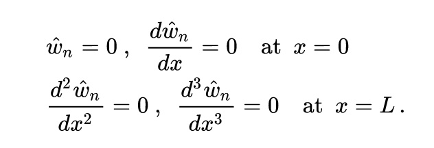
The top line states that: at \(x=0\), the bottom of the fork, our beam does not travel away from its natural axis (yes, because its a solid hunk of metal connected to the base), and it does not deflect (slope).
The bottom line stats that: at \(x=L\), the top of the fork is straight (which is true, the tip-top of the fork does indeed not bend, only the middleish parts bend.)
So, to get at the hidden system of four elements, we will take some derivatives of our original \(\hat{w}(x)\) equation by \(x\), as prescribed by our initial conditions.
wp = diff(w,x,1)
wpp = diff(w,x,2)
wppp = diff(w,x,3)
(wp, wpp, wppp)
(b*d3*cos(b*x) + b*d1*cosh(b*x) - b*d2*sin(b*x) + b*d0*sinh(b*x),
 -b^2*d2*cos(b*x) + b^2*d0*cosh(b*x) - b^2*d3*sin(b*x) + b^2*d1*sinh(b*x),
 -b^3*d3*cos(b*x) + b^3*d1*cosh(b*x) + b^3*d2*sin(b*x) + b^3*d0*sinh(b*x))
And then, we have a system:
cond_1 = w.subs(x=0) == 0
cond_2 = wp.subs(x=0) == 0
cond_3 = wpp.subs(x=L) == 0
cond_4 = wppp.subs(x=L) == 0

conds = (cond_1, cond_2, cond_3, cond_4)
conds
(d0 + d2 == 0,
 b*d1 + b*d3 == 0,
 -b^2*d2*cos(L*b) + b^2*d0*cosh(L*b) - b^2*d3*sin(L*b) + b^2*d1*sinh(L*b) == 0,
 -b^3*d3*cos(L*b) + b^3*d1*cosh(L*b) + b^3*d2*sin(L*b) + b^3*d0*sinh(L*b) == 0)
solve(conds, d0, d1, d2, d3).full_simplify()
Ok so, we notice that out of all of these boundary expressions the \(b^{n}\) term drop out. Therefore, we have the system:
\begin{equation} \begin{cases} d_0 + d_2 = 0 \\ d_1 + d_3 = 0 \\ -d_2 \cos L\beta + d_0 \cosh L\beta - d_3 \sin L\beta + d_1 \sinh L\beta = 0 \\ -d_3 \cos L\beta + d_1 \cosh L\beta + d_2 \sin L\beta + d_0 \sinh L\beta = 0 \\ \end{cases} \end{equation}
Great. Four unknowns, four equations. We can now figure out when a solution for \(d_0, \dots d_3\) exists (or go about solving it, but turns out that’s significantly harder and wildly useless.)
I will spare you the pages of route algebra needed to figure out when a solution exists. Suffice to say its lots of trig identities.
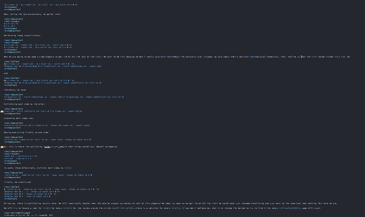
But, the satisfying conclusion is that, given the equations above, a solution exists for \(d_0 \dots d_3\) (read: a mode for the beam exists), when:
\begin{equation} \cos L\beta \cdot \cosh L\beta +1 = 0 \end{equation}
So, any valid solutions for the expression \(\cos x \cdot \cosh x + 1 = 0\) will be a valid product between \(L\beta\). We can use this information to figure out the right frequencies by then solving for \(f\) embedded in \(\beta\).
So, onto solving for \(\cos L\beta \cdot \cosh L\beta +1 = 0\).
We again give up and ask a computer to do it.We will try to locate a root for \(Lb\) for every \(\pi\) for two rounds around the circle (until \(4 \pi\))—there is a solution for every \(\pi\), if you don’t believe me, plot it or change the bottom to try to find it for every \(\frac{\pi}{2}\), sage will crash:
intervals = [jj*pi for jj in range(0, 5)]
intervals
[0, pi, 2*pi, 3*pi, 4*pi]
We will now declare \(x=L\beta\), and create a nonlinear expression in it:
x = var("x")
characteristic_eqn = 1 + cos(x)*cosh(x) == 0
characteristic_eqn
cos(x)*cosh(x) + 1 == 0
Root finding time!
characteristic_solutions = [characteristic_eqn.find_root(i,j) for (i,j) in zip(intervals,intervals[1:])]
characteristic_solutions
[1.8751040687120917, 4.6940911329739246, 7.854757438237603, 10.995540734875457]
These are possible candidate values for \(L\beta\). We will declare these values \(s\).
So, we now have that:
\begin{equation} L \beta = s \end{equation}
Substituting back our original definition for \(\beta\), we have that:
\begin{equation} L \sqrt{2\pi f} \qty(\frac{u}{EI})^{\frac{1}{4}} = s \end{equation}
Now, we will try to get \(f\) by itself:
\begin{align} &L \sqrt{2\pi f} \qty(\frac{u}{EI})^{\frac{1}{4}} = s \\ \Rightarrow\ & \sqrt{2\pi f} = \frac{s}{L} \qty(\frac{EI}{u})^{\frac{1}{4}} \\ \Rightarrow\ & 2\pi f = \frac{s^{2}}{L^{2}} \qty(\frac{EI}{u})^{\frac{1}{2}} \\ \Rightarrow\ & f = \frac{s^{2}}{2\pi L^{2}} \qty(\frac{EI}{u})^{\frac{1}{2}} \end{align}
Finally, we have that \(I = \frac{1}{12} bh^{3}\) for a rectangular prism; and that linear density is cross-sectional area times volumetric density \(\mu = \rho \cdot bh\). Making these substitutions:
\begin{align} f &= \frac{s^{2}}{2\pi L^{2}} \qty(\frac{EI}{u})^{\frac{1}{2}} \\ &= \frac{s^{2}}{2\pi L^{2}} \qty(\frac{Ebh^{3}}{12 \rho bh})^{\frac{1}{2}} \\ &= \frac{s^{2}}{2\pi L^{2}} \qty(\frac{Eh^{2}}{12 \rho})^{\frac{1}{2}} \\ \end{align}
Without even getting to the frequency-based payoff, we immediately notice two takeaways.
- The frequency of our fork is inversely proportional to length (i.e. \(f = \frac{1}{L^{2}}\dots\))
- The first overtone of the tuning fork is \(s^{2} = (\frac{4.694}{1.875})^{2} \approx 6.27\) times higher than the fundamental—meaning its significantly higher energy so it dissipates significantly faster; it is also not an integer multiple, which means its much less likely to be confused to be a harmonic; making a tuning fork essentially a pure-frequency oscillator
- Given equal conditions, only the thickness in one dimension (the one perpendicular to the bending axis) matters
But, enough idling, onto our main event. Using standard reference values for aluminum, as well as our measured length and thickness of a \(C’\ 512hz\) tuning fork, we have that
# measured values----
# thickness
h = 0.0065 # meters
# length
L0 = 0.09373 # meters
L1 = 0.08496 # meters

# theoretical values---
# elastic modulus
E = 46203293995 # pascals = kg/m^2
# density
p = 2597 # kg/m^3

# our solved characteristic value (s)
# mode to index
nth_mode = 0
s = characteristic_solutions[nth_mode]

zero = (((s^2)/(2*pi*L0^2))*((E*h^2)/(12*p))^(1/2)).n()
one = (((s^2)/(2*pi*L1^2))*((E*h^2)/(12*p))^(1/2)).n()

zero, one

mean([zero,one])
(504.123425101814, 613.571395642254)
558.847410372034
Close enough for a night. Thank you sorry about everything.
temperature
# mode to index
nth_mode = 0
# s = characteristic_solutions[nth_mode]
s = var("s")

# change to L and h (distances measures) by increases in degrees C
d(t,x) = (2.4e-5)*x
rho(t,x) = ((2.4e-5))*x
a,b = var("a b")
# a = -3.9
# b = 0.0033
Ed(t) = ((a*b)*e^(b*t))*1e9

f(E, L, h, p) = (((s^2)/(2*pi*L^2))*((E*h^2)/(12*p))^(1/2))

E,L,h,p = var("E L h p")

# (a * b * /g)c

t = var("t")

# diff(t, dt, E,L,h,p) = sqrt((f.diff(E)*Ed(t)*dt)^2 + (f.diff(E)*Ed(t)*dt)^2 + (f.diff(L)*d(t)*dt)^2 + (f.diff(h)*d(t)*dt)^2)
# diff(10, 1, 42661456706, 0.09833, 0.00643, 2545.454545).n()

subdict = {
a: -3.9, b:0.0033, L:0.09833, h:0.00643, p:2545.454545, E:42661456706, s:characteristic_solutions[nth_mode], t:50
}

(f.diff(E)*Ed(t)).subs(subdict).full_simplify().n()
(f.diff(L)*d(t,L)).subs(subdict).full_simplify().n()
(f.diff(h)*d(t,h)).subs(subdict).full_simplify().n()
(f.diff(p)*rho(t,p)).subs(subdict).full_simplify().n()
-0.0782394489394635
-0.0211103561467420
0.0105551780733710
-0.00527758903668550
expansion = var("x")
l,w,h,m = var("l w h m")
density(l,w,h) = (l*w*h)/m
density.diff(l)*expansion + density.diff(w)*expansion + density.diff(h)*expansion
(l, w, h) |--> h*l*x/m + h*w*x/m + l*w*x/m