For an ODE, eigensolutions of some expression \(x’=Ax\) consists of the class of solutions which remains in a line through the origin, which consists of the family which:
\begin{equation} x(t) = ke^{\lambda t} v \end{equation}
where \(\lambda\) is an eigenvalue of \(A\), and \(v\) its corresponding eigenvector.
motivation
\begin{equation} y’ = F(y) \end{equation}
an autonomous ODE, suppose we have some solution \(y=a\) for which \(y’ = 0\), that is, \(F(a) = 0\), we know that the system will be trapped there.
Near such a stationary solution \(a\), we can use a Taylor expansion to linearize:
\begin{equation} F(a+b) = F(a) + Jac(a)x + \dots \end{equation}
The first term, we are given, is \(0\). The second term indicates that our derivative near the stationary point seems to be some matrix \(A\) of \(a\).
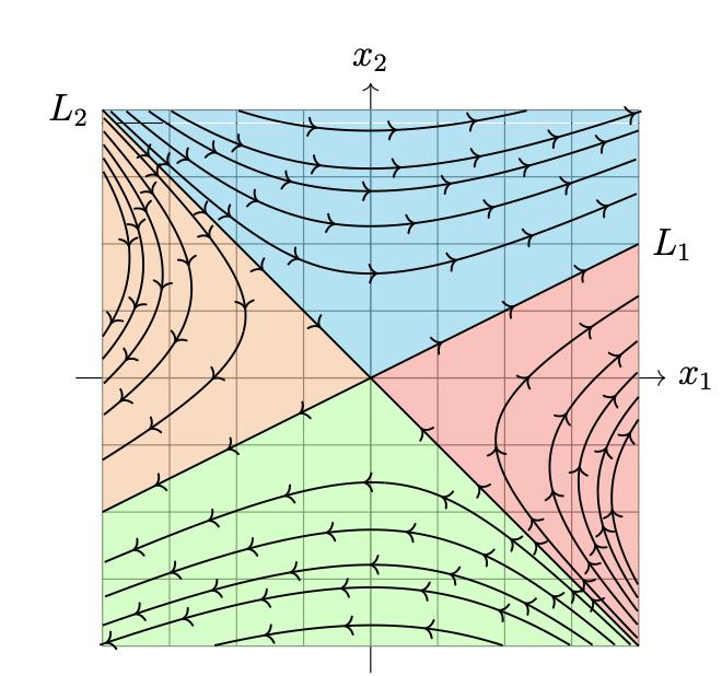
sketching solutions along eigenlines
For eigenlines, we can observe the sign of the eigenline to see how it behaves, and—in conjuction—how other solutions behave. In particular, in the x1, x2 plane for two orders, the solutions are tangent to the eigensolutions.
With an negative eigenvalue, the eigensolution arrows will point towards the origin, whereas with positive eigenvalues the eigensolutions will point away.
- saddle case: if \(\lambda_{1}\) and \(\lambda_{2}\) have opposite signs, then the paths look like half-parabolas matching the eigensolutions; it will approach the larger eigenvalue more rapidly
- node/source/sink case: if \(\lambda_{1}\) and \(\lambda_{2}\) have the same sign, then the solutions look like half-parabolas tangent only to the eigenline which has a smaller \(\lambda\) — in this case, if the eigenvalues happens to be both negative you can work things out for \(-A\) and then flip the paths on all the lines—at smaller values of \(t\) (specifically \(t<1\)), the curve tends closer to the \(\lambda\) with the smaller eigenvalue (because raising the power to a larger number actually makes the power smaller); at \(t>1\), the curve moves towards that of the bigger eigenvalue
- complex/spiral case: in this case, we can write some answer with Euler’s Equation to get two real solutions in trig \(P(t) + iQ(t)\), where each \(P,Q\) is some function is cos plus sin times \(ae^{t}\). Therefore, it will be a spiral outwards
Flipping
You will note that, in all of these cases \(x=0\) is a stationary solution, as \(A0 = 0\). As \(t \to -\infty\), we end up kissing the side with the smaller eigenvalue, and as \(t \to +\infty\), we end up going towards the side with the bigger eigenvalue.
Nonlinear
Non-linear systems can be figured by the motivation above, linearizing into groups, and figuring out each local area.
Flipping
This is because:
\begin{equation} (-A)v = -(Av) = (-\lambda) v \end{equation}
meaning the directions of eigenvectors don’t change while their corresponding eigenvalues change. If we define some \(y(t) = x(-t)\), where \(Ax = x’\), we can work out that \(y’(t) = -Ay(t)\), meaning that \(y’\)’s graphs are just flipped versions of \(x\)’s graphs.
Hence we can just flip everything.
Drawing
By tracing those patterns, you can draw other solutions over time: