The Euler-Bernoulli Theory is a theory in dynamics which describes how much a beam deflect given an applied load.
Assumptions
For Euler-Bernoulli Theory to apply in its basic form, we make assumptions.
- The “beam” you are bending is modeled as a 1d object; it is only long and is not wide
- For this page, \(+x\) is “right”, \(+y\) is “in”, and \(+z\) is “up”
- Probably more, but we only have this so far.
- the general form of the Euler-Bernoulli Theory assumes a freestanding beam
Basic Statement
The most basic for the Euler-Bernoulli Equation looks like this:
\begin{equation} \dv[2]x \qty(EI\dv[2]{w}{x}) =q(x) \end{equation}
where, \(w(x)\) is the deflection of the beam at some direction \(z\) at position \(x\). \(q\) is the load distribution (force per unit length, similar to pressure which is force per unit area, at each point \(x\)). \(E\) is the Elastic Modulus of the beam, and \(I\) the second moment of area of the beam’s cross section.
Note that \(I\) must be calculated with respect to the axis perpendicular to the load. So, for a beam placed longside by the \(x\) axis, and pressed down on the \(z\) axis, \(I\) should be calculated as: \(\iint z^{2}\dd{y}\dd{z}\).
Pretty much all the time, the Elastic Modulus \(E\) (how rigid your thing is) and second moment of area \(I\) (how distributed are the cross-section’s mass) are constant; therefore, we factor them out, making:
\begin{align} &\dv[2]x \qty(EI\dv[2]{w}{x}) =q(x) \\ \Rightarrow\ & EI \qty(\dv[2]x \dv[2]{w}{x} )=q(x) \\ \Rightarrow\ & EI \dv[4]{w}{x} = q(x) \end{align}
This is also apparently used everywhere in engineering to figure out how bendy something will be given some \(q\) put along the beam.
Ok, let’s take the original form of this equation and take some integrals to see the edges of this thing:
\begin{equation} \dv[2]{x} \qty(EI \dv[2]{w}{x}) = q(x) \end{equation}
First things first, let’s take a single integral:
\begin{equation} \dv{x} \qty(EI \dv[2]{w}{x}) = -Q \end{equation}
This is the total shear force on the material (the sum of all forces applied to all points \(\int q(x)\).) We have a sign difference
old notes
Let’s take some transverse load \(q(x,t)\), applied at time \(t\) at location \(x\). To model the load/bending/vibration of the rod, we first have to know a few more things.
First, figure the Young’s Modulus \(E\) of the thing that you are bending.
Of course, we also want to know what shape our thing is; more specifically, we want to know how the point masses in our thing is distributed. So we will also need the second moment of area \(I\).
Finally, we should have \(m\) mass per unit length of the rod we are bending.
The Euler-Bernoulli Theory tells us that the deflection (distance from the neutral-axis) each point \(x\) in the material should get is:
\begin{equation} EI \pdv[4]{w}{x} + m \pdv[2]{w}{t} = q(x,t) \end{equation}
Solving this lovely Differential Equation would tell you how far away each point diverges from the neutral point.
Tracing this out over \((x,t)\), we can get some trace of how the thing vibrates by measuring the behavior of \(\omega\).
free vibrations in Euler-Bernoulli Theory
If no time-varying \(q\) exists, we then have:
\begin{equation} EI \pdv[4]{w}{x} + m \pdv[2]{w}{t} = 0 \end{equation}
And then some magical Differential Equations happen. I hope to learn them soon.
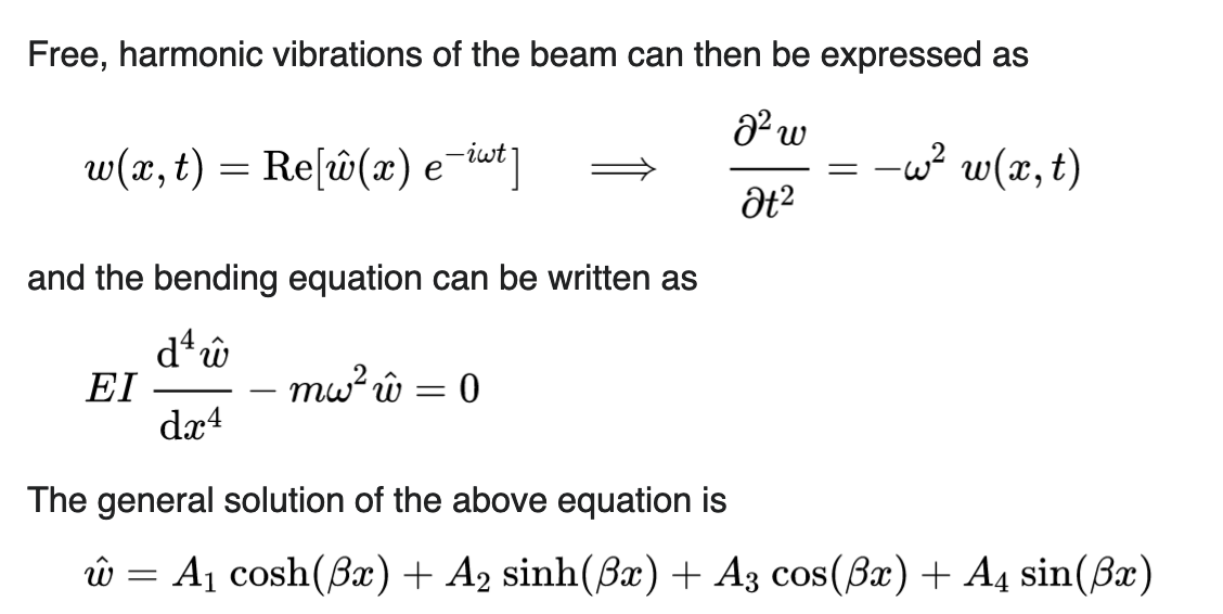
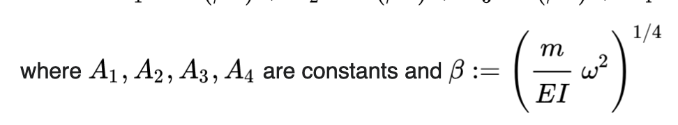
The result here is significant: if we can figure the actual rate of vibrations which we expect.
However, this doesn’t really decay—but funing torks do. How?
Apparently because air resistance—Zachary Sayyah. So Sasha time.