filters are how beliefs are updated from observation
discrete state filter
\begin{equation} b’(s’) = P(s’|b,a,o) \end{equation}
\(b’\) is what state we think we are in next, and its a probability distribution over all states, calculated given from \(b,a,o\) our current belief about our state, our action, and our observation.
We can perform this belief update by performing Bayes Theorem over \(o\):
\begin{align} b’(s’) &= P(s’|b,a,o) \\ &\propto P(o|b,a,s’) P(s’ | b,a) \end{align}
Now, consider
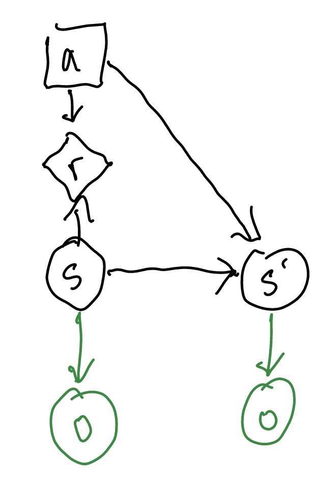
\(b\) is a representation of \(s\) (“belief is a representation of what previous state you are in.”) However, you will note that \(s\) is conditionally independent to \(o\) through d-seperation as there is a chain \(s \to s’ \to o\). So:
\begin{align} b’(s’) &\propto P(o|b,a,s’) P(s’ | b,a) \\ &= P(o|a,s’) P(s’ | b,a) \end{align}
This first term is by definition the observation model, so we have:
\begin{align} b’(s’) &\propto P(o|a,s’) P(s’ | b,a) \\ &= O(o|a,s’)P(s’ | b,a) \end{align}
We now invoke the law of total probability over the second term, over all states:
\begin{align} b’(s’) &\propto O(o|a,s’)P(s’ | b,a) \\ &= O(o|a,s’) \sum_{s}^{} P(s’|b,a,s)P(s|b,a) \end{align}
If we know \(s\) and \(a\) in the \(P(s’|b,a,s)\) terms, we can drop \(b\) because if we already know \(a,s\) knowing what probability we are in \(s\) (i.e. \(b(s)\)) is lame. Furthermore, \(P(s|b,a)=b(s)\) because the action we take is irrelavent to what CURRENT state we are in, if we already are given a distribution about what state we are in through \(b\).
\begin{align} b’(s’) &\propto O(o|a,s’) \sum_{s}^{} T(s’|s,a)b(s) \end{align}
Kalman Filter
A Kalman Filter is a continous state-filter where by each of our \(T, O, b\) is represented via a Gaussian distribution. Kalman Filter is discrete state filter but continuous. Consider the final, belief-updating result of the discrete state filter above, and port it to be continous:
\begin{equation} b’(s’) \propto O(o|a,s’) \int_{s} T(s’|s,a) b(s) ds \end{equation}
if we modeled our transition probabilties, observations, and initial belief with a gaussian whereby each parameter is a gaussian model parameterized upon a few matricies.
\begin{equation} T(s’|s,a) = \mathcal{N}(s’|T_{s} s + T_{a} a, \Sigma_{s}) \end{equation}
\begin{equation} O(o|s’) = \mathcal{N}(o|O_{s}s’, \Sigma_{o}) \end{equation}
\begin{equation} b(s) = \mathcal{N}(s | \mu_{b}, \Sigma_{b}) \end{equation}
where, \(T, O\) are matricies that maps vectors states to vectors. \(\Sigma\) are covariances matricies. Finally, \(\mu\) is a mean belief vector.
Two main steps:
predict
\begin{equation} \mu_{p} \leftarrow T_{s} \mu_{b} + T_{a}a \end{equation}
\begin{equation} \Sigma_{p} \leftarrow T_{s} \Sigma_{b} T_{s}^{T} + \Sigma_{s} \end{equation}
given our current belief \(b\) and its parameters, and our current situation \(s,a\), we want to make a prediction about where we should be next. We should be somewhere on: \(b’_{p} = \mathcal{N}(\mu_{p}, \Sigma_{p})\).
update
\begin{equation} \mu_{b} \leftarrow \mu_{p}+K(o-O_{s}\mu_{p}) \end{equation}
\begin{equation} \Sigma_{b} \leftarrow (I-KO_{s})\Sigma_{p} \end{equation}
where \(K\) is Kalmain gain
We are now going to take an observation \(o\), and update our belief about where we should be now given our new observation.
Kalmain gain
\begin{equation} K \leftarrow \Sigma_{p} O_{s}^{T} (O_{s}\Sigma_{p}O_{s}^{T}+\Sigma_{O})^{-1}} \end{equation}
Additional Information
Extended Kalman Filter
Kalman Filter, but no linearity required by forcing linearity by a point-jacobian estimate about the mean of the belief state.
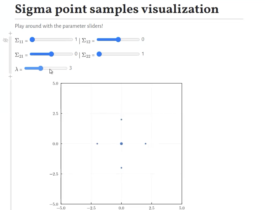
Unscented Kalman Filter
its Extended Kalman Filter but derivative free, which means its clean and hence its unscented.
Its achieved through using “sigma point samples”: just taking some representative points (mean + 2 points in each direction), and draw a line.
Particle Filter
Its a filter with Likelihood Weighted Sampling.
Say we are flying a plane; we want to use our height measures to infer our horizontal location. Let us take an observation model: \(O(o|s,a) = \mathcal{N}(o|h(s), \sigma)\) (“the probability of getting an observation given we are in the state”)
- start off with a prior distribution over the states you have: a distribution over the possible states
- make \(N\) monte-calro samples from our prior. These are our particles.
- use the transition model to propagate the \(N\) samples forward to get \(N\) new next-state samples
- take action \(a\); calculate \(O(o|s,a)\) for each of your proper gated samples \(s\) (“how likely is our observed altitude given each of our sampled states?”)
- normalise the resulting probabilities into a single distribution
- re-sample \(N\) samples that from the resulting distribution. these are our updated belief.
- repeat from step 3
main pitfalls: if we don’t have enough sampled particles, you may get condensations that doesn’t make sense
particle filter with rejection
This is used almost never but if you really want to you can. You’d get a bunch of particles and take an action. You propagate the particles forward.
For each propergated state \(s\), if what you observed \(o\) is equal to (or close to, for continuous cases) \(sample(o|s,a)\), you keep it around. Otherwise, you discard it.
You keep doing this until you have kept enough states to do this again, and repeat.
Injection particle filter
Add a random new particle every so often to prevent particle deprivation.
Adaptive injection particle filter
We perform injection based on the ratio of two moving averages of particle weights—if all weights are too low, we chuck in some to perturb it