requirements
Consider a function that has no periodicity, but that:
\begin{equation} f(x), -\infty < x < \infty \end{equation}
And assume that:
\begin{equation} \int_{\infty}^{\infty} |f(x)| \dd{x}, < \infty \end{equation}
important: look up! the integral of \(f(x)\) has to converge AND this means that the \(f(x)\) goes to \(0\) actually at boundaries.
(meaning the function decays as you go towards the end)
definition
a Fourier transform is an invertible transformation:
\begin{equation} f(x) \to \hat{f}(\lambda) \end{equation}
and
\begin{equation} \hat{f}(\lambda) \to f(x) \end{equation}
Where,
\begin{equation} \hat{f}(\lambda) = \int_{-\infty}^{\infty } e^{-i\lambda x} f(x) \dd{x} \end{equation}
\begin{equation} f(x) = \frac{1}{2\pi} \int_{\infty}^{-\infty} e^{ix\lambda} \hat{f}(\lambda) \dd{\lambda} \end{equation}
We sometimes write:
\begin{equation} \hat{f}(\lambda) = \mathcal{F}(f)(\lambda) \end{equation}
where \(\mathcal{F}\) is an invertible map that gives you the Fourier Series.
additional information
Properties of \(\mathcal{F}\)
- it’s a Linear Map: \(\mathcal{F}(c_1 f_1 + c_2 f_2) = c_1\mathcal{F}(f_1) + c_2 \mathcal{F}(f_2)\)
- it’s recenter able: \(\mathcal{F}(f(x+c)) = e^{i c \lambda}\mathcal{F}(f)(\lambda)\)
- it’s reverse-shift-able: \(\mathcal{F}\qty(e^{i \lambda_{0} x} f(x)) = \mathcal{F}(f) (\lambda -\lambda_{0})\)
Proof:
- because integrals are linear
- \(\int_{-\infty}^{\lambda} e^{-i(t-c)\lambda}f(t) \dd{t} = e^{ic\lambda} \mathcal{F}(f)(\lambda)\), where we define \(t = x+c\)
- try it
Derivative of Fourier Transform
Suppose we want:
\begin{equation} \mathcal{F}(f’(x)) = \int_{\infty}^{\infty} e^{-ix\lambda} f’(x) \dd{x} = \left e^{-ix\lambda} f(x)\right|_{-\infty}^{\infty} + i \lambda \int_{-\infty}^{\infty} e^{-ix\lambda} f(x) \dd{x} = i \lambda \mathcal{F}(f) (\lambda) \end{equation}
Because we are guaranteed \(f(x)\) evaluated at infinity is \(0\), the first term drops out. The important conclusion here: *Fourier transforms change a derivative into ALGEBRA of multiplying by \(i\lambda\).
Consider also:
\begin{equation} \mathcal{F}(x f(x)) = i \dv \lambda \mathcal{F}(f)(\lambda) \end{equation}
you can show this in a similar way, by attempting to distribute a \(\dv \lambda\) into the Fourier transform and showing that they are equal.
Fourier Transform of a Gaussian
\begin{equation} \mathcal{F}\qty(e^{-\frac{ax^{2}}{2}}) = \sqrt{\frac{2\pi}{a}}e^{-\frac{\lambda^{2}}{2a}} \end{equation}
and:
\begin{equation} \mathcal{F}^{-1}\qty(e^{-a\frac{\lambda^{2}}{2}}) = \frac{e^{-\frac{x^{2}}{2a}}}{\sqrt{2\pi a}} \end{equation}
we obtain this:
\begin{equation} u = e^{-\frac{x^{2}}{2}} \end{equation}
and:
\begin{equation} \dv{u}{x} = -xe^{-\frac{x^{2}}{2}} = -xu \end{equation}
and if we took a Fourier transform on both sides, we obtain:
\begin{equation} \mathcal{F}\qty(\dv{u}{x} + xu) = 0 = i \lambda \hat{u} + i \pdv{\hat{u}} = 0 \end{equation}
and note that this is the same equation. Meaning:
\begin{equation} \mathcal{F}\qty(\dv{u}{x} + xu) = \dv{\lambda}{x} + \lambda u \end{equation}
this gives:
\begin{equation} \mathcal{F}(u) = Cu \end{equation}
which is what we see.
Look! A table
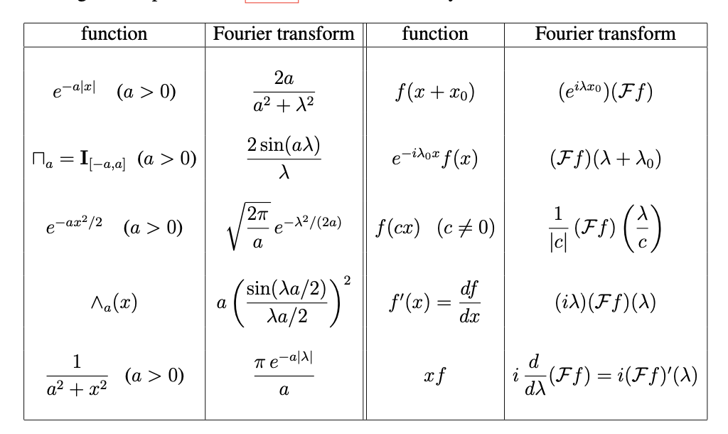
where:
\begin{equation} \Lambda_{a} \end{equation}
is the triangle between \([-a, a]\), that goes up to \(1\).
interpreting \(\lambda\)
if \(f(x)\) is a function in time
\(\lambda\) could be thought of analogous to frequency
if \(f(x)\) is a function of space
\(\lambda\) could be thought of analogous to momentum
Fourier transform of step function
if you have a function:
\begin{equation} f(x) = \begin{cases} 1, |x| < a \\ 0 \end{cases} \end{equation}
its Fourier transform is sinc function:
\begin{equation} \hat{f}(\lambda) = \frac{i \sin (a \lambda)}{\lambda} \end{equation}
intuitive understandings the formula
sines stuck between
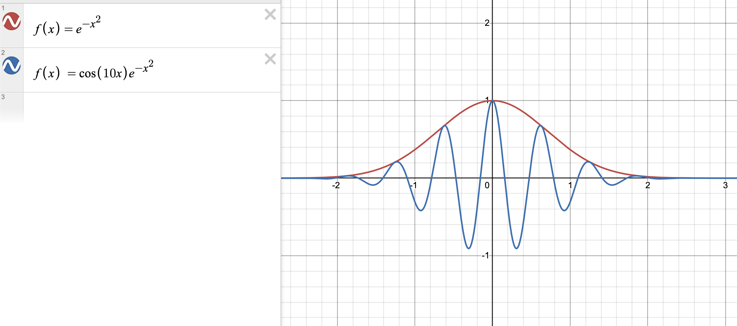
Consider what:
\begin{equation} f(x) \cos (x) \end{equation}
looks like.
Effectively, you are stenching the \(\cos(x)\) between \(f(x)\) and its reflection across \(x\). As you integrate, the majority of the up and downs cancel out, and the only thing you are left is the bits where \(f(x)\) peak up!
as you increase \(k\):
\begin{equation} f(x) \cos (kx) \end{equation}
you obtain more cancellations and it will eventually integrate to \(0\).
Fourier transform properties
As a function gets smoother, its Fourier transform is more concentrated at one point (closer to a single frequency).
Conversely, as a function gets more jagged, its Fourier transform is smoother (closer to a composition of sinusoids).
Fourier Transform as Quantization
Consider:
the big fun idea—-we can transform:
- \(L\) periodic function on \(f(x)\)
- \(\left\{ (c_{n})^{\infty}_{-\infty} \right\}\)
This series exists for all function, converges exceedingly quickly, and has great properties. It should look like the form:
\begin{equation} f(x) = \sum_{-\infty}^{\infty} c_{n} e^{n \omega x i} \end{equation}
Fourier norm of a function
After you do this, and obtain
\(\left\{ (c_{n})^{\infty}_{-\infty} \right\}\)
we call the “size” of this function:
\begin{equation} \sum_{-\infty}^{\infty} | c_{n}|^{2} \end{equation}
Planchrel’s Formula
For a usual \(L\) periodic function, size agrees:
\begin{equation} \langle f,f \rangle= \int_{0}^{L} |f(x)|^{2} \dd{x} = L\sum_{-\infty}^{\infty} | c_{n}|^{2} \end{equation}
You can show this by plugging in the Complex Fourier Series in \(f\).
motivation
Consider a function period of period \(L\)
\begin{equation} a_{k} = \int_{0}^{L} F(x) e^{-i\omega kx} \dd{x} \end{equation}
where:
\begin{equation} f(x) = ?\sum_{k} a_{n} e^{i \omega kx} \end{equation}
And the BIG PICTURE: if we took the period \(L \to \infty\), we end up with the Fourier Transform.