A memo from the administrators at Metropolis Health System, in response to a nationwide blood shortage, asked the care teams and doctors at all of their hospitals to be particularly conservative and judicious in how they used blood products because of the critical shortage. Phoebe, a 17-year-old girl, is being treated for leukemia at Metro Hospital, which is part of the health system. She has gone through several rounds of chemotherapy, but has not responded to the treatment.
Her oncologist does not think further chemotherapy will benefit her, and only likely harm her. Her care team has discussed with Phoebe and her parents that they do not recommend further treatment, and instead think the focus should be on providing comfort and pain relief for her in her remaining months of life. Phoebe and her parents agree. Phoebe’s hemoglobin is low, and the team has been providing regular blood transfusions to help her feel better, but without any hemorrhaging site noted. In light of the blood shortage, Phoebe’s treatment team is concerned about whether the blood transfusions are an appropriate use of a scarce resource.
Metro Hospital is a busy urban hospital with at least several trauma cases daily that require blood products. They also are aware of patients such as Felix, a 19-year-old, who has sickle cell disease who also needs routine blood transfusions.
Phoebe’s team is wanting consultation on how to approach these issues of being stewards of a scarce resource, and balancing the importance of pain-relief and palliative care with the needs of other patients – as well as considering that the blood shortages also impact patients in other hospitals
this is NOT futility
- will this patient ever stop needing top level of care?
- are they enjoying and benefiting from the treatment
- allocation
ethical guidelines
- respect for persons
- beneficence
- justice
what is just? in praticular especially due to strotage? “hopsitals as allocators”
affirmative action
“no action with one hand tied behind my back”
=> real harm
counterargument: beneficence
…but the tangible benfits are palliative and there exists other types of pallative support
recommendatino
- prioriteze others, follow hopsital guidelens for baseline
- if there are left over, administer care
Like a sound you hear That lingers in your ear But you can’t forget From sundown to sunset
It’s all in the air You hear it everywhere No matter what you do It’s gonna grab a hold on you California soul
\begin{equation} x_1^{(j)} = x_1^{(j-1)} + Attn\qty(x_{k}^{(j-1)}, \forall k) \end{equation}
\begin{equation} At_{x_{1}^{(j-1)}} = \text{softmax}\qty(\frac{q_{1} k_{j}, \forall j}{\sqrt{d_{\ \text{model}}}}) v_{j} \end{equation}
\begin{equation} At_{x_{1}^{(j-1)}} = \text{softmax}_{\text{top-k cliff}}\qty(\frac{q_{1} k_{j}, \forall j}{\sqrt{d_{\ \text{model}}}}) v_{j} \end{equation}
- obtaining a function for the gradient of policy against some parameters \(\theta\)
- making them more based than they are right now by optimization
Thoughout all of this, \(U(\theta)\) is \(U(\pi_{\theta})\).
Obtaining a policy gradient
Finite-Difference Gradient Estimation
We want some expression for:
\begin{equation} \nabla U(\theta) = \qty[\pdv{U}{\theta_{1}} (\theta), \dots, \pdv{U}{\theta_{n}}] \end{equation}
we can estimate that with the finite-difference “epsilon trick”:
\begin{equation} \nabla U(\theta) = \qty[ \frac{U(\theta + \delta e^{1}) - U(\theta)}{\delta} , \dots, \frac{U(\theta + \delta e^{n}) - U(\theta)}{\delta} ] \end{equation}
where \(e^{j}\) is the standard basis vector at position \(j\). We essentially add a small \(\delta\) to the \(j\) th slot of each parameter \(\theta_{j}\), and divide to get an estimate of the gradient.
Linear Regression Gradient Estimate
We perform \(m\) random perturbations of \(\theta\) parameters, and lay each resulting parameter vector flat onto a matrix:
\begin{equation} \Delta \theta = \mqty[(\Delta \theta^{1})^{T} \\ \dots \\ (\Delta \theta^{m})^{T}] \end{equation}
For \(\theta\) that contains \(n\) parameters, this is a matrix \(m\times n\).
We can now write out the \(\Delta U\) with:
\begin{equation} \Delta U = \qty[U(\theta+ \Delta \theta^{1}) - U(\theta), \dots, U(\theta+ \Delta \theta^{m}) - U(\theta)] \end{equation}
We have to compute Roll-out utility for each \(U(\theta + …)\)
We now want to fit a function between \(\Delta \theta\) to \(\Delta U\), because from the definition of the gradient we have:
\begin{equation} \Delta U = \nabla_{\theta} U(\theta)\ \Delta \theta \end{equation}
(that is \(y = mx\))
Rearranging the expression above
\begin{equation} \nabla_{\theta} U(\theta) \approx \Delta \theta^{\dagger} \Delta U \end{equation}
where \(\Delta \theta^{\dagger}\) is the pseudoinverse of \(\Delta \theta\) matrix.
To end up at a gradient estimate.
Likelyhood Ratio Gradient
This is likely good, but requires a few things:
- an explicit transition model that you can compute over
- you being able to take the gradient of the policy
this is what people usually refers to as “Policy Gradient”.
Recall:
\begin{align} U(\pi_{\theta}) &= \mathbb{E}[R(\tau)] \\ &= \int_{\tau} p_{\pi} (\tau) R(\tau) d\tau \end{align}
Now consider:
\begin{align} \nabla_{\theta} U(\theta) &= \int_{\tau} \nabla_{\theta} p_{\pi}(\tau) R(\tau) d \tau \\ &= \int_{\tau} \frac{p_{\pi} (\tau)}{p_{\pi} (\tau)} \nabla_{\tau} p_{\tau}(\tau) R(\tau) d \tau \end{align}
Aside 1:
Now, consider the expression:
\begin{equation} \nabla \log p_{\pi} (\tau) = \frac{\nabla p_{\pi}(\tau)}{p_{\pi} \tau} \end{equation}
This is just out of calculus. Consider the derivative chain rule; now, the derivative of \(\log (x) = \frac{1}{x}\) , and the derivative of the inside is \(\nabla x\).
Rearranging that, we have:
\begin{equation} \nabla p_{\pi}(\tau) = (\nabla \log p_{\pi} (\tau))(p_{\pi} \tau) \end{equation}
Substituting that in, one of our \(p_{\pi}(\tau)\) cancels out, and, we have:
\begin{equation} \int_{\tau} p_{\pi}(\tau) \nabla_{\theta} \log p_{\pi}(\tau) R(\tau) \dd{\tau} \end{equation}
You will note that this is the definition of the expectation of the right half (everything to the right of \(\nabla_{\theta}\)) vis a vi all \(\tau\) (multiplying it by \(p(\tau)\)). Therefore:
\begin{equation} \nabla_{\theta} U(\theta) = \mathbb{E}_{\tau} [\nabla_{\theta} \log p_{\pi}(\tau) R(\tau)] \end{equation}
Aside 2:
Recall that \(\tau\) a trajectory is a pair of \(s_1, a_1, …, s_{n}, a_{d}\).
We want to come up with some \(p_{\pi}(\tau)\), “what’s the probability of a trajectory happening given a policy”.
\begin{equation} p_{\pi}(\tau) = p(s^{1}) \prod_{k=1}^{d} p(s^{k+1} | s^{k}, a^{k}) \pi_{\theta} (a^{k}|s^{k}) \end{equation}
(“probably of being at a state, times probability of the transition happening, times the probability of the action happening, so on, so on”)
Now, taking the log of it causes the product to become a summation:
\begin{equation} \log p_{\pi}(\tau) = p(s^{1}) + \sum_{k=1}^{d} p(s^{k+1} | s^{k}, a^{k}) + \pi_{\theta} (a^{k}|s^{k}) \end{equation}
Plugging this into our expectation equation:
\begin{equation} \nabla_{\theta} U(\theta) = \mathbb{E}_{\tau} \qty[\nabla_{\theta} \qty(p(s^{1}) + \sum_{k=1}^{d} p(s^{k+1} | s^{k}, a^{k}) + \pi_{\theta} (a^{k}|s^{k})) R(\tau)] \end{equation}
This is an important result. You will note that \(p(s^{1})\) and \(p(s^{k+1}|s^{k},a^{k})\) doesn’t have a \(\theta\) term in them!!!!. Therefore, taking term in them!!!!*. Therefore, taking the \(\nabla_{\theta}\) of them becomes… ZERO!!! Therefore:
\begin{equation} \nabla_{\theta} U(\theta) = \mathbb{E}_{\tau} \qty[\qty(0 + \sum_{k=1}^{d} 0 + \nabla_{\theta} \pi_{\theta} (a^{k}|s^{k})) R(\tau)] \end{equation}
So based. We now have:
\begin{equation} \nabla_{\theta} U(\theta) = \mathbb{E}_{\tau} \qty[\sum_{k=1}^{d} \nabla_{\theta} \log \pi_{\theta}(a^{k}|s^{k}) R(\tau)] \end{equation}
where,
\begin{equation} R(\tau) = \sum_{k=1}^{d} r_{k}\ \gamma^{k-1} \end{equation}
“this is very nice” because we do not need to know anything regarding the transition model. This means we don’t actually need to know what \(p(s^{k+1}|s^{k}a^{k})\) because that term just dropped out of the gradient.
We can simulate a few trajectories; calculate the gradient, and average them to end up with our overall gradient.
Reward-to-Go
Variance typically increases with Rollout depth. We don’t want that. We want to correct for the causality of action/reward. Action in the FUTURE do not influence reward in the PAST.
Recall:
\begin{equation} R(\tau) = \sum_{k=1}^{d} r_{k}\ \gamma^{k-1} \end{equation}
Let us plug this into the policy gradient expression:
\begin{equation} \nabla_{\theta} U(\theta) = \mathbb{E}_{\tau} \qty[\sum_{k=1}^{d} \nabla_{\theta} \log \pi_{\theta}(a^{k}|s^{k}) \qty(\sum_{k=1}^{d} r_{k}\ \gamma^{k-1})] \end{equation}
Let us split this reward into two piece; one piece for the past (up to \(k-1\)), and one for the future:
\begin{equation} \nabla_{\theta} U(\theta) = \mathbb{E}_{\tau} \qty[\sum_{k=1}^{d} \nabla_{\theta} \log \pi_{\theta}(a^{k}|s^{k}) \qty(\sum_{l=1}^{k-1} r_{l}\ \gamma^{l-1} + \sum_{l=k}^{d} r_{l}\ \gamma^{l-1})] \end{equation}
We now want to ignore all the past rewards (i.e. the first half of the internal summation). Again, this is because action in the future shouldn’t care about what reward was gather in the past.
\begin{equation} \nabla_{\theta} U(\theta) = \mathbb{E}_{\tau} \qty[\sum_{k=1}^{d} \nabla_{\theta} \log \pi_{\theta}(a^{k}|s^{k}) \sum_{l=k}^{d} r_{l}\ \gamma^{l-1}] \end{equation}
We now factor out \(\gamma^{k-1}\) to make the expression look like:
\begin{equation} \nabla_{\theta} U(\theta) = \mathbb{E}_{\tau} \qty[\sum_{k=1}^{d} \nabla_{\theta} \log \pi_{\theta}(a^{k}|s^{k}) \qty(\gamma^{k-1} \sum_{l=k}^{d} r_{l}\ \gamma^{l-k})] \end{equation}
We call the right term Reward-to-Go:
\begin{equation} r_{togo}(k) = \sum_{l=k}^{d} r_{l}\ \gamma^{l-k} \end{equation}
where \(d\) is the depth of your trajectory and \(k\) is your current state. Finally, then:
\begin{equation} \nabla_{\theta} U(\theta) = \mathbb{E}_{\tau} \qty[\sum_{k=1}^{d} \nabla_{\theta} \log \pi_{\theta}(a^{k}|s^{k}) \qty(\gamma^{k-1} r_{togo}(k))] \end{equation}
Baseline subtraction
Sometimes, we want to subtract a baseline reward to show how much actually better an action is (instead of blindly summing all future rewards). This could be the average reward at all actions at that state, this could be any other thing of your choosing.
\begin{equation} \nabla_{\theta} U(\theta) = \mathbb{E}_{\tau} \qty[\sum_{k=1}^{d} \nabla_{\theta} \log \pi_{\theta}(a^{k}|s^{k}) \qty(\gamma^{k-1} (r_{togo}(k) - r_{baseline}(k)))] \end{equation}
For instance, if you have a system where each action all gave \(+1000\) reward, taking any particular action isn’t actually very good. Hence:
Optimizing the Policy Gradient
We want to make \(U(\theta)\) real big. We have two knobs: what is our objective function, and what is your restriction?
Policy Gradient Ascent
good ‘ol fashioned
\begin{equation} \theta \leftarrow \theta + \alpha \nabla U(\theta) \end{equation}
where \(\alpha\) is learning rate/step factor. This is not your STEP SIZE. If you want to specify a step size, see Restricted Step Method.
Restricted Step Method
Policy Gradient Ascent can take very large steps if the gradient is too large.
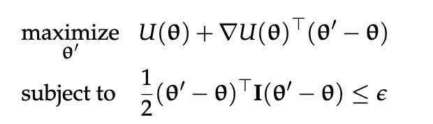
One by which we can optimize the gradient, ensuring that we don’t take steps larger than:
\begin{equation} \frac{1}{2}(\theta’ - \theta)^{T} I(\theta’ - \theta) \leq \epsilon \end{equation}
is through Restricted Gradient:
\begin{equation} \theta \leftarrow \theta + \sqrt{2 \epsilon} \frac{\nabla U(\theta)}{|| \nabla U(\theta)||} \end{equation}
Occasionally, if a step-size is directly given to you in terms of euclidean distance, then you would replace the entirety of \(\sqrt{2 \epsilon}\) with your provided step size.
Trust Region Policy Optimization
Using a different way of restricting the update.
Proximal Policy Optimization
Clipping the gradients.
plan
actions:
- dive (check of a subquestion to the plan)
- swipe (read a new document to answer the question)
- replan (reset stack with a new query that’s not the previous one)
- answer (stop diving, answer the question) eusnotuh eoue
mmmm
mmm
The depolarizing channel can be represented using the Kraus operators provided. For a quantum state \(\rho\), the action of the depolarizing channel \(E\) can be expressed using the Kraus representation as:
\[ E(\rho) = \sum_{i=0}^{n} A_i \rho A_i^\dagger \]
In your case, you mentioned three Kraus operators corresponding to the depolarizing channel. Given the Kraus operators:
\[ A_0 = \sqrt{1 - \frac{3p}{4}} \quad A_1 = \sqrt{\frac{p}{4}} X \quad A_2 = \sqrt{\frac{p}{4}} Y \quad A_3 = \sqrt{\frac{p}{4}} Z \]
We can substitute these into the Kraus representation. The action of the depolarizing channel \(E\) on the state \(\rho\) will be:
\[ E(\rho) = A_0 \rho A_0^\dagger + A_1 \rho A_1^\dagger + A_2 \rho A_2^\dagger + A_3 \rho A_3^\dagger \]
Now, substituting in the expressions for the Kraus operators, we get:
\[ E(\rho) = \left( \sqrt{1 - \frac{3p}{4}} \, \rho \, \sqrt{1 - \frac{3p}{4}} \right) + \left( \frac{p}{4} \, X \rho X \right) + \left( \frac{p}{4} \, Y \rho Y \right) + \left( \frac{p}{4} \, Z \rho Z \right) \]
Thus, the correct Kraus representation of the depolarizing channel operation \(E(\rho)\) in terms of the given probabilities and Kraus operators is:
\[ E(\rho) = \left( 1 - \frac{3p}{4} \right) \rho + \frac{p}{4} X \rho X + \frac{p}{4} Y \rho Y + \frac{p}{4} Z \rho Z \]
This formula describes how the channel affects the state \(\rho\) considering the defined noise strength \(p\).
\begin{equation} E(\rho)=(1-p)\rho+\frac{p}{3}X\rho X+\frac{p}{3}Y\rho Y+\frac{p}{3}Z\rho Z \end{equation}
\begin{equation} E(\rho)=(1-p)\rho+\frac{p}{3}X\rho X+\frac{p}{3}Y\rho Y+\frac{p}{3}Z\rho Z \end{equation}
\begin{equation} E(\rho) = \left( 1 - \frac{3p}{4} \right) \rho + \frac{p}{4} X \rho X + \frac{p}{4} Y \rho Y + \frac{p}{4} Z \rho Z \end{equation}
\begin{equation} \sqrt{\frac{x^{3}}{y+z}} \end{equation}
\begin{equation} \frac{1}{\frac{y}{x} + \frac{z}{x}} \end{equation}
\begin{equation} x\qty(\frac{x}{y+z}) \end{equation}
osnethuaoeu
aoensuthaoeu
tnoehu choneu o osnetuh
anstehu
\begin{equation} \frac{1}{2} \end{equation}
\begin{equation} \frac{12}{3} \sum_{k=1}^{n} \int \end{equation}
\begin{align} \min_{x}\quad & \frac{1}{2}x^{2} \\ \textrm{s.t.} \quad & x \geq 0 \\ & x^{2} \norm{12}_{x} \end{align}
\begin{align} \qty {\frac{1}{2} \qty(\frac{12}{323})} \end{align}
\begin{equation} \mqty(1 & 2 & 3 \\ 4 & 5 & 6) \end{equation}
| ansoteuh | asnoethu | aontseuh |
|---|---|---|
| sanotehu | asnotehu | aoeu |
| snoetuh | ||
| \(\frac{3}{3}\) | ||
| oeunsht | ||
| ntoaehusnaotehusntahoeusnth | ||
1+3
4
12/322 + 234 /23
10.211180124223603
Consider the term we have for attention scores:
\begin{equation} \text{softmax}\qty(\frac{Q^{(k)} K^{(k)}^{T} + \ones \log \qty(P^{(k)})^{T}}{\sqrt{d_{\ \text{model}}}) \end{equation}
Now, let’s consider each element \(i,j\) from the softmax. That gives:
\begin{equation} \frac{e^{q^{(k)}_{i}^{T} \cdot k^{(k)}_{j} + \log \qty(P^{(k)})_{j}}}{\sum_{j} e^{q^{(k)}_{i}^{T} \cdot k^{(k)}_{j} + \ones \log \qty(P^{(k)})_{j}}} \end{equation}
Notice that by exponents, we have
\begin{equation} \frac{e^{\log \qty(P^{(k)})_{j}}}e^{q^{(k)}_{i}^{T} \cdot k^{(k)}_{j}}{\sum_{j} e^{q^{(k)}_{i}^{T} \cdot k^{(k)}_{j} + \ones \log \qty(P^{(k)})_{j}}} \end{equation}
which is
\begin{equation} \frac{P^{(k)}_{j}e^{q^{(k)}_{i}^{T} \cdot k^{(k)}_{j}}{\sum_{j} e^{q^{(k)}_{i}^{T} \cdot k^{(k)}_{j} + \ones \log \qty(P^{(k)})_{j}}} \end{equation}
exactly a multiplicative scale on the attention indexed to keys.
We will add the following analysis of FLOPs to our article. We note in particular that the FLOPs analysis support our notion of training for half of the amount of tokens as a reasonable computation bound on FLOP-matching use.
In terms of the training FLOPs; let \(d\) be our hidden dimension and \(L\) be the block size:
- attention projections costs \(6Ld^{2}\)
- output projection costs \(2Ld^{2}\)
- attention itself is quadratic in \(2L^{2}d\)
- MLP for \(16 Ld^{2}\)
The only mechanism is a forking projection, which maps inputs \(L \times D\) to \(d \times 2\) map, with the convention that multiplications counts as one pass and addition counts as another, we obtain that the forking projection costs \(4Ld\).
Let the forking model’s block size be \(kL\). Thus the training performance ratio would be:
\begin{equation} \frac{24 Ld^{2} + 4L^{2}d}{24 k Ld^{2} + 4k^{2}L^{2}d + 4kLd} = \frac{6d+L}{k \qty(6d + kl + 1)} \end{equation}
setting \(d=2048, L=512, K = 2\), this would be around \(0.481\), which as expected is around 2 times worth of inefficiency.
In terms of inference time FLOPs, a reasonable upper-bound would be