Using Linear Regression to perform a classification task \(y \in \qty {0,1}\) sounds kind of silly. We assume that \(y\) follows a kind of Bernoulli distribution.
requirements
\begin{align} h_{\theta}\qty(x) &= g\qty(\theta^{T} x) \\ &= \frac{1}{1+e^{-\theta^{T}x}} \end{align}
That is, we apply a sigmoid function to our linear regression output to perform classification. Such a sigmoid function has the following properties:
\begin{equation} p\qty(y=1|x;\theta) = h_{\theta}\qty(x) \end{equation}
\begin{equation} p\qty(y=0|x;\theta) = 1-h_{\theta}\qty(x) \end{equation}
\begin{equation} y \in \qty {0,1} \end{equation}
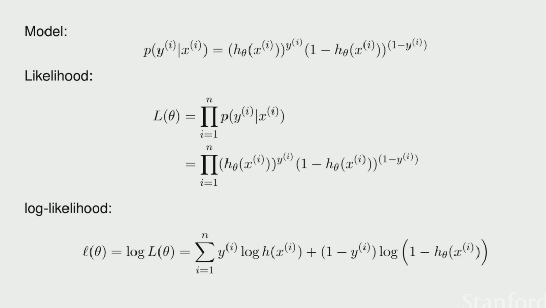
\begin{equation} p\qty(y|x; \theta) = h_{\theta} \qty(x)^{y} \qty(1-h_{\theta}\qty(x))^{1-y} \end{equation}
likelihood function
To perform MLE to find best fit \(\theta\), we can write:
\begin{align} L\qty(\theta) &= \prod_{i=1}^{n} P\qty(y^{(i)} | x^{(i)}; \theta) \\ &= \prod_{i=1}^{n} h_{\theta}\qty(x^{(i)})^{y(i)} \qty(1-h_{\theta}\qty(x^{(i)}))^{1-y^{(i)}} \end{align}
Taking the log of this expression to turn this into a sum:
\begin{equation} l\qty(\theta) = \sum_{i=1}^{n} y^{(i)} \log h\qty(x^{(i)}) + \qty(1-y^{(i)}) \log \qty(1-h_{\theta}\qty(x^{(i)})) \end{equation}
Consider now if we take the derivative of this and perform a close-form solution:
\begin{equation} \theta_{j} = \theta_{j} + \alpha \sum_{i=1}^{n} \qty(y^{(i)} - h_{\theta}\qty(x^{(i)})) x_{j}^{(i)} \end{equation}
additional information
Probabilistic Motivation of logistic regression
Naive Bayes acts to compute \(P(Y|X)\) via the Bayes rule and using the Naive Bayes assumption. What if we can model the value of \(P(Y|X)\) directly?
With \(\sigma\) as the sigmoid function:
\begin{equation} P(Y=1|X=x) = \sigma (\theta^{\top}x) \end{equation}
and we tune the parameters of \(\theta\) until this looks correct.
We always want to introduce a BIAS parameter, which acts as an offset; meaning the first \(x\) should always be \(1\), which makes the first value in \(\theta\) as a “bias”.
For optimizing this function, we have:
\begin{equation} LL(\theta) = y \log \sigma(\theta^{\top} x) + (1-y) \log (1- \theta^{\top} x) \end{equation}
and if we took the derivative w.r.t. a particular parameter slot \(\theta_{j}\):
\begin{equation} \pdv{LL(\theta)}{\theta_{j}} = \sum_{i=1}^{n} \qty[y^{(i)} - \sigma(\theta^{\top}x^{(i)})] x_{j}^{(i)} \end{equation}
logistic regression assumption
We assume that there exists that there are some \(\theta\) which, when multiplied to the input and squashed by th sigmoid function, can model our underlying probability distribution:
\begin{equation} \begin{cases} P(Y=1|X=x) = \sigma (\theta^{\top}x) \\ P(Y=0|X=x) = 1- \sigma (\theta^{\top}x) \\ \end{cases} \end{equation}
We then attempt to compute a set of \(\theta\) which:
\begin{equation} \theta_{MLE} = \arg\max_{\theta} P(y^{(1)}, \dots, y^{(n)} | \theta, x_1 \dots x_{n}) \end{equation}
Log Likelihood of Logistic Regression
To actually perform MLE for the $θ$s, we need to do parameter learning. Now, recall that we defined, though the logistic regression assumption:
\begin{equation} P(Y=1|X=x) = \sigma (\theta^{\top}x) \end{equation}
essentially, this is a Bernouli:
\begin{equation} (Y|X=x) \sim Bern(p=\sigma(\theta^{\top}x)) \end{equation}
We desire to maximize:
\begin{equation} P(Y=y | \theta, X=x) \end{equation}
Now, recall the continous PDF of Bernouli:
\begin{equation} P(Y=y) = p^{y} (1-p)^{1-y} \end{equation}
we now plug in our expression for \(p\):
\begin{equation} P(Y=y|X=x) = \sigma(\theta^{\top}x)^{y} (1-\sigma(\theta^{\top}x))^{1-y} \end{equation}
for all \(x,y\).
Logistic Regression, in general
For some input, output pair, \((x,y)\), we map each input \(x^{(i)}\) into a vector of length \(n\) where \(x^{(i)}_{1} … x^{(i)}_{n}\).
Training
We are going to learn weights \(w\) and \(b\) using stochastic gradient descent; and measure our performance using cross-entropy loss
Test
Given a test example \(x\), we compute \(p(y|x)\) for each \(y\), returning the label with the highest probability.
Logistic Regression Text Classification
Given a series of input/output pairs of text to labels, we want to assign a predicted class to a new input fair.
We represent each text in terms of features. Each feature \(x_{i}\) comes with some weight \(w_{i}\), informing us of the importance of feature \(x_{i}\).
So: input is a vector \(x_1 … x_{n}\), and some weights \(w_1 … w_{n}\), which will eventually gives us an output.
There is usually also a bias term \(b\). Eventually, classification gives:
\begin{equation} z = w \cdot x + b \end{equation}
However, this does not give a probability, which by default this does not. To fix this, we apply a squishing function \(\sigma\), which gives
\begin{equation} \sigma(z) = \frac{1}{1+\exp(-z)} \end{equation}
which ultimately yields:
\begin{equation} z = \sigma(w \cdot x+ b) \end{equation}
with the sigmoid function.
To make this sum to \(1\), we write:
\begin{equation} p(y=1|x) = \sigma(w \cdot x + b) \end{equation}
and
\begin{equation} p(y=0|x) = 1- p(y=1|x) \end{equation}
Also, recall that \(\sigma(-x) = 1- \sigma(x)\), this gives:
\begin{equation} p(y=0|x) = \sigma(-w\cdot x-b) \end{equation}
the probability at which point we make a decision is called a decision boundary. Typically this is 0.5.
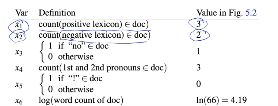
We can featurize by counts from a lexicon, by word counts, etc.
For instance:
logistic regression terms
- feature representation: each input \(x\) is represented by a vectorized lit of feature
- classification function: \(p(y|x)\), computing \(y\) using the estimated class
- objective function: the loss to minimize (i.e. cross entropy)
- optimizer: SGD, etc.
- decision boundary: the threshold at which classification decisions are made, with \(P(y=1|x) > N\).
binary cross entropy
\begin{equation} \mathcal{L} = - \qty[y \log \sigmoid(w \cdot x + b) + (1-y) \log (1- \sigmoid(w \cdot x + b))] \end{equation}
or, for neural networks in general:
\begin{equation} \mathcal{L} = - \qty[y \log \hat{y} + (1-y) \log (1- \hat{y})] \end{equation}
Weight gradient for logistic regresison
\begin{equation} \pdv{L_{CE}(\hat(y), y)}{w_{j}} = \qty[\sigma\qty(w \cdot x + b) -y] x_{j} \end{equation}
where \(x_{j}\) is feature \(j\).