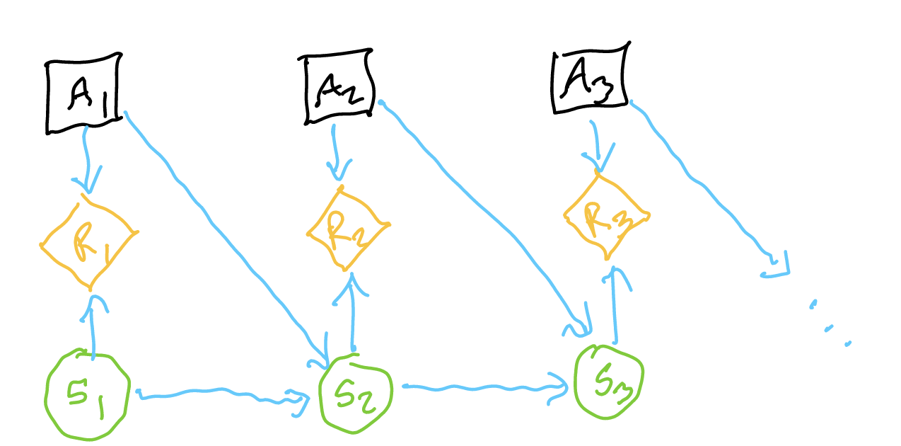
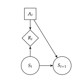
A MDP is a decision network whereby a sequences of actions causes a sequence of states. Each state is dependent on the action we take and the state we are in, and each utility is dependent on action taken and the state we are in.
Note that, unlike a POMDP, we know what state we are in—the observations from the states are just unclear.
constituents
- \(S\): state space (assuming discrete for now, there are \(n\) states) — “minimum set of information that allows you to solve a problem”
- \(A\): action space — set of things your agent can do
- \(T(s’ | s,a)\): “dynamics”, state-transition model “probability that we end up in \(s’\) given \(s\) and action \(a\)”: good idea to make a table of probabilities of source vs. destination variables
- \(R(s,a,s’)\): expected reward given in an action and a state (real world reward maybe stochastic)
- \(\pi_{t}(s_{1:t}, a_{1:t-1})\): the policy, returning an action, a system of assigning actions based on states
- however, our past states are d-seperated from our current action given knowing the state, so really we have \(\pi_{t}(s_{t})\)
additional information
We assume policy to be exact right now.
stationary Markov Decision Process
This is a stationary Markov Decision Process because at each node \(S_{n}\), we have: \(P(S_{n+1} | A_n, S_n)\). Time is not a variable: as long as you know what state you are in, and what you did, you know the transition probability.
(that is, the set of states is not dependent on time)
calculating utility with instantaneous rewards
Because, typically, in decision networks you sum all the utilities together, you’d think that we should sum the utilities together.
finite-horizon models
We want to maximize reward over time, over a finite horizon \(n\). Therefore, we try to maximize:
\begin{equation} \sum_{t=1}^{n}r_{t} \end{equation}
this function is typically called “return”.
infinite-horizon models
If you lived forever, small positive \(r_{t}\) and large \(r_{t}\) makes no utility difference. We therefore add discounting:
\begin{equation} \sum_{t=1}^{\infty} \gamma^{t-1} r_{t} \end{equation}
where, \(\gamma \in (0,1)\)
we discount the future by some amount—an “interest rate”—reward now is better than reward in the future.
- \(\gamma \to 0\): “myopic” strategies, near-sighted strategies
- \(\gamma \to 1\): “non-discounting”
average return models
We don’t care about this as much:
\begin{equation} \lim_{n \to \infty} \frac{1}{n} \sum_{t=1}^{n}r_{t} \end{equation}
but its close to infinite-horizon models with Gama close to \(1\)
Solving an MDP
You are handed or can predict \(R(s,a)\), and know all transitions
Small, Discrete State Space
Get an exact solution for \(U^{*}(s)\) (and hence \(\pi^{ *}(a, s)\)) for the problem via…
Large, Continuous State Space
Parameterize Policy
Optimize \(\pi_{\theta}\) to maximize \(U(\pi_{\theta})\) using Policy Optimization methods!
Gradient Free: lower dimension policy space
Gradient Based Method: higher dimension policy space
Parameterize Value Function
Optimize \(U_{\theta}(S)\) via global approximation or local approximation methods, then use a greedy policy on that nice and optimized value function.
You can only reason about your immediate surroundings/local reachable states
or… “you don’t know the model whatsoever”
during these cases, you never argmax over all actions; hence, its important to remember the methods to preserve Exploration and Exploitation.