MCVI solves POMDPs with continuous state space, but with discrete observation and action spaces. It does this by formulating a POMDP as a graph.
Fast algorithms require discretized state spaces, which makes the problem much more difficult to model. MCVI makes continuous representations possible for complex domains.
MC Backup
Normal POMDP Bellman Backup isn’t going to work well with continuous state spaces.
Therefore, we reformulate our value backup as:
\begin{equation} V_{t+1}(b) = \max_{a \in A} \qty(\int_{s} R(s,a)b(s) \dd{s}) + \gamma \sum_{o \in O}^{} p(o|b,a) V_{t}(update(b,a,o)) \end{equation}
whereby, a continuous belief update:
\begin{equation} update(b,a,o) = \kappa O(o|s’,a) \int_{s \in S} T(s’|s,a) b(s) \dd{s} \end{equation}
where \(\kappa\) is a normalisation constant to keep the new belief a probability.
But! Instead of actually taking the integral, we simulate a series of trajectories and sum the toal reward
MC-Backup at Graph
We construct at graph by sticking each best action determined by rolling out \(L\) steps and computing the reward.
Collecting the values given each observation, we create a new node for the best action; the best action per observation is connected as well.
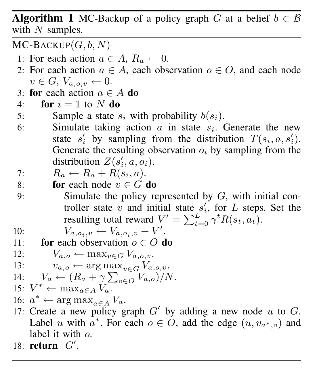
This creates a new optimal policy graph from the rollouts.
MCVI
- initial each reward at action to \(0\)
- for each observation, initialize each observation, node as \(0\)
- Take monte-carlo samples across the actions and states to take integrals to obtain:
- \(HV_{g}(b) = \max_{a \in A} \qty(\int_{s \in S} R(s,a)b(s) \dd{s} + \sum_{o}^{} ???)\)
- each future observation is sampled using monte-carlo simulation
each backup, you pick one new node to add.