Naive Bayes is a special class of Baysian Network inference problem which follows a specific structure used to solve classification problems.
The Naive Bayes classifier is a Baysian Network of the shape:
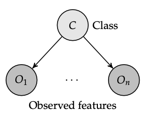
(Why is this backwards(ish)? Though we typically think about models as a function M(obs) = cls, the real world is almost kind of opposite; it kinda works like World(thing happening) = things we observe. Therefore, the observations are a RESULT of the class happening.)
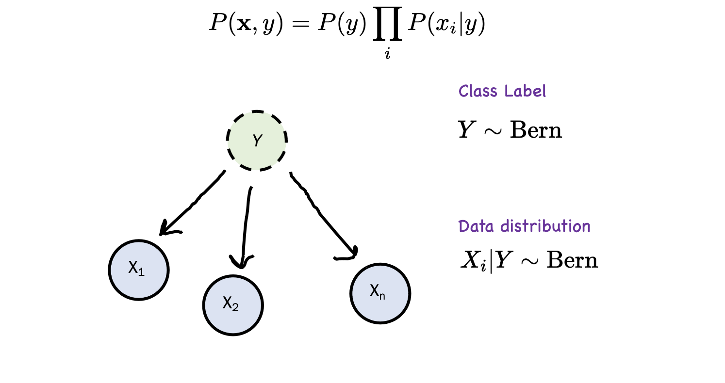
We consider, naively, \(o_{1:n}\) are all conditionally independent on \(c\). From this graph, we can therefore use the probability chain rule + conditional probability to write that:
\begin{equation} P(c, o_{1:n}) = P( c) \prod_{i=1}^{n} P(o_{i} | c) \end{equation}
so, to actually compute this, we don’t want to bother going over all the multiplications because of underflow, we write:
\begin{equation} \hat{y} = \arg\max_{y} \log \hat{P}(y) + \sum_{i=1}^{m} \log \hat{P}(x|y) \end{equation}
brute-force Bayes classifier
\begin{equation} \arg\max_{y} P(y|x) = \arg\max_{y} \frac{P(x|y)P(y)}{P(x)} \end{equation}
but because we are taking argmax, we can not normalize:
\begin{equation} \arg\max_{y} P(y|x) = \arg\max_{y} P(x|y)P(y) \end{equation}
this only works if \(x\) is a single value (i.e. you have a one-feature classifier
This system has 6 parameters; they can be MLE for Bernouli from data, but you can also use Baysian Parameter Learning Method
| y = 0 | y = 1 | |
|---|---|---|
| x1 = 0 | theta0 | theta2 |
| x1 = 1 | theta1 | theta3 |
| y = 0 | |
|---|---|
| y = 0 | theta4 |
| y = 1 | theta5 (=1-theta4) |
to perform estiimation with MAP
\begin{equation} p(X=1| Y=0) = \frac{\text{examples where X=1, Y=0}}{\text{examples where Y=0}} \end{equation}
whith MLE with a Laplace prior:
\begin{equation} p(X=1| Y=0) = \frac{\text{(examples where X=1, Y=0)}+1}{\text{(examples where Y=0)}+\text{(nclass = 2)}} \end{equation}
We can keep going; for instance, if you wave \(x_1, x_2\) two diffferent features:
\begin{equation} \arg\max_{y} P(y|x) = \arg\max_{y} P(x_1, x_2|y)P(y) \end{equation}
but this requires us to have \(2^{2}\) and ultimately \(2^{n}\) parameters, which is exponential blowup. Hence, we need to treat the variables as—naivly—independent so we can multiply them. Hence:
Naive Bayes assumption
we assume independence between the input features. That is, we assume:
\begin{equation} P(x_1, \dots, x_{n}|y) = \prod_{i=1}^{n} P(X_{i}|y) \end{equation}
inference with Naive Bayes
Recall the definition of inference, for our case here:
given observations \(o_{1:n}\), we desire to know what’s the probability of \(c\) happening. That is, from conditional probability:
\begin{equation} P(c | o_{1:n}) = \frac{P(c, o_{1:n})}{P(o_{1:n})} \end{equation}
Now, from above we have \(P(c, o_{1:n})\) already. To get the denominator, we invoke law of total probability to add up the probability of all observations occurring given all classes. That is:
\begin{equation} P(o_{1:n}) = \sum_{c \in C} P(c, o_{1:n}) \end{equation}
You will note that this value \(P(o_{1:n})\) is actually constant as long as the network structure does not change. Therefore, we tend to write:
\begin{align} P(c | o_{1:n}) &= \frac{P(c, o_{1:n})}{P(o_{1:n})} \\ &= \kappa P(c, o_{1:n}) \end{align}
or, that:
\begin{equation} P(c|o_{1:n}) \propto P(c, o_{1:n}) \end{equation}
“the probability of a class occurring given the inputs is proportional to the probability of that class occurring along with the inputs”
Multiple believes
\begin{equation} P(A=a | R_1) \propto P(R_1 | A=a) \cdot P(A=a) \end{equation}
But now
Motivation: Bayes rule
This will give us:
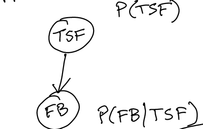
However, what if we don’t want to use the law of total probability to add up \(P(FB’)\)?
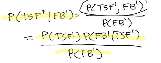
We can actually write a relation that essentially reminds us that the fact that \(P(FB’)\) as not dependent on \(TSF\), so we can write:
\begin{equation} P(TSF^{1}|FB^{1}) \porpto P(TSF^{1})P(FB^{1} | TSF^{1}) \end{equation}