Here’s the characteristic equation again:
\begin{equation} \pdv[2] x \qty(EI \pdv[2]{w}{x}) = -\mu \pdv{w}{t}+q(x) \end{equation}
After Fourier decomposition, we have that:
\begin{equation} EI \dv[4]{\hat{w}}{x} - \mu f^{2}\hat{w} = 0 \end{equation}
Let’s solve this!
E,I,u,f = var("E I u f")
x, L = var("x L")
w = function('w')(x)
_c0, _c1, _c2, _c3 = var("_C0 _C1 _C2 _C3")
fourier_cantileaver = (E*I*diff(w, x, 2) - u*f^2*w == 0)
fourier_cantileaver
-f^2*u*w(x) + E*I*diff(w(x), x, x) == 0
And now, we can go about solving this result.
solution = desolve(fourier_cantileaver, w, ivar=x, algorithm="fricas").expand()
w = solution
\begin{equation} _{C_{1}} e^{\left(\sqrt{f} x \left(\frac{u}{E I}\right)^{\frac{1}{4}}\right)} + _{C_{0}} e^{\left(i \, \sqrt{f} x \left(\frac{u}{E I}\right)^{\frac{1}{4}}\right)} + _{C_{2}} e^{\left(-i \, \sqrt{f} x \left(\frac{u}{E I}\right)^{\frac{1}{4}}\right)} + _{C_{3}} e^{\left(-\sqrt{f} x \left(\frac{u}{E I}\right)^{\frac{1}{4}}\right)} \end{equation}
We will simplify the repeated, constant top of this expression into a single variable \(b\):
b = var("b")
top = sqrt(f)*(u/(E*I))**(1/4)

w = _c1*e^(b*x) + _c0*e^(i*b*x) + _c2*e^(-i*b*x) + _c3*e^(-b*x)
w
_C1*e^(b*x) + _C0*e^(I*b*x) + _C2*e^(-I*b*x) + _C3*e^(-b*x)
\begin{equation} _{C_{1}} e^{\left(b x\right)} + _{C_{0}} e^{\left(i \, b x\right)} + _{C_{2}} e^{\left(-i \, b x\right)} + _{C_{3}} e^{\left(-b x\right)} \end{equation}
We have one equation, four unknowns. However, we are not yet done. We will make one more simplifying assumption—try to get the \(e^{x}\) into sinusoidal form. We know this is supposed to oscillate, and it being in sinusoidal makes the process of solving for periodic solutions easier.
Recall that:
\begin{equation} \begin{cases} \cosh x = \frac{e^{x}+e^{-x}}{2} \\ \cos x = \frac{e^{ix}+e^{-ix}}{2}\\ \sinh x = \frac{e^{x}-e^{-x}}{2} \\ \sin x = \frac{e^{ix}-e^{-ix}}{2i}\\ \end{cases} \end{equation}
With a new set of scaling constants \(d_0\dots d_3\), and some rearranging, we can rewrite the above expressions into just a linear combination of those elements. That is, the same expression for \(w(x)\) at a specific frequency can be written as:
\begin{equation} d_0\cosh bx +d_1\sinh bx +d_2\cos bx +d_3\sin bx = w \end{equation}
No more imaginaries!!
So, let us redefine the expression:
d0, d1, d2, d3 = var("d0 d1 d2 d3")
w = d0*cosh(b*x)+d1*sinh(b*x)+d2*cos(b*x)+d3*sin(b*x)
w
d2*cos(b*x) + d0*cosh(b*x) + d3*sin(b*x) + d1*sinh(b*x)
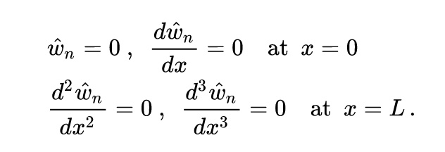
Now, we need to move onto solving when there will be valid solutions to this expression. However, we currently have four unknowns, and only one equation (at \(x=0\), \(w=0\), because the cantilever is fixed at base); so, to get a system in four elements, we will take some derivatives.
The way that we will go about this is by taking three derivatives and supplying the following initial conditions to get four equations:
wp = diff(w,x,1)
wpp = diff(w,x,2)
wppp = diff(w,x,3)
(wp, wpp, wppp)
(b*d3*cos(b*x) + b*d1*cosh(b*x) - b*d2*sin(b*x) + b*d0*sinh(b*x),
 -b^2*d2*cos(b*x) + b^2*d0*cosh(b*x) - b^2*d3*sin(b*x) + b^2*d1*sinh(b*x),
 -b^3*d3*cos(b*x) + b^3*d1*cosh(b*x) + b^3*d2*sin(b*x) + b^3*d0*sinh(b*x))
And then, we have a system:
cond_1 = w.subs(x=0) == 0
cond_2 = wp.subs(x=0) == 0
cond_3 = wpp.subs(x=L) == 0
cond_4 = wppp.subs(x=L) == 0

conds = (cond_1, cond_2, cond_3, cond_4)
conds
(d0 + d2 == 0,
 b*d1 + b*d3 == 0,
 -b^2*d2*cos(L*b) + b^2*d0*cosh(L*b) - b^2*d3*sin(L*b) + b^2*d1*sinh(L*b) == 0,
 -b^3*d3*cos(L*b) + b^3*d1*cosh(L*b) + b^3*d2*sin(L*b) + b^3*d0*sinh(L*b) == 0)
solve(conds, d0, d1, d2, d3).full_simplify()
Ok so, we notice that out of all of these boundary expressions the \(b^{n}\) term drop out. Therefore, we have the system:
\begin{equation} \begin{cases} d_0 + d_2 = 0 \\ d_1 + d_3 = 0 \\ -d_2 \cos Lb + d_0 \cosh Lb - d_3 \sin Lb + d_1 \sinh Lb = 0 \\ -d_3 \cos Lb + d_1 \cosh Lb + d_2 \sin Lb + d_0 \sinh Lb = 0 \\ \end{cases} \end{equation}
Now, taking the top expressions, we gather that:
\begin{equation} \begin{cases} d_0 = -d_2 \\ d_1 = -d_3 \end{cases} \end{equation}
Performing these substitutions:
\begin{equation} \begin{cases} d_0 (\cos Lb + \cosh Lb) + d_1 (\sin Lb + \sinh Lb) = 0 \\ d_1 (\cos Lb + \cosh Lb) + d_0 (\sinh Lb- \sin Lb ) = 0 \\ \end{cases} \end{equation}
Now we are going to do some cursed algebra to get rid of all the rest of the \(d\). We want to do this because we don’t really care much what the constants are; instead, we care about when a solution exists (hopefully, then, telling us what the \(f\) baked inside \(b\) is). So:
\begin{align} &d_0 (\cos Lb + \cosh Lb) + d_1 (\sin Lb + \sinh Lb) = 0 \\ \Rightarrow\ & \frac{-d_0}{d_1} = \frac{(\sin Lb + \sinh Lb)}{(\cos Lb + \cosh Lb)} \end{align}
and
\begin{align} &d_1 (\cos Lb + \cosh Lb) + d_0 (\sinh Lb- \sin Lb ) = 0 \\ \Rightarrow\ & \frac{-d_0}{d_1} = \frac{(\cos Lb + \cosh Lb)}{(\sinh Lb- \sin Lb )} \end{align}
therefore, we have:
\begin{equation} \frac{(\sin Lb + \sinh Lb)}{(\cos Lb + \cosh Lb)} = \frac{(\cos Lb + \cosh Lb)}{(\sinh Lb- \sin Lb )} \end{equation}
Multiplying each side by the other:
\begin{equation} (\sin Lb + \sinh Lb)(\sinh Lb- \sin Lb ) = (\cos Lb + \cosh Lb)^{2} \end{equation}
Expanding both sides now:
\begin{equation} (\sinh^{2} Lb-\sin^{2} Lb) = (\cos^{2} Lb + 2\cos Lb\ \cosh Lb + \cosh ^{2}Lb) \end{equation}
Moving everything finally to one side:
\begin{equation} \sinh^{2} Lb - \cosh^{2} Lb -\sin ^{2} Lb - \cos ^{2}Lb - 2\cos Lb \cosh Lb = 0 \end{equation}
Ok, this is where the satisfying “candy crush” begins when things cancel out. Recall pythagoras:
\begin{equation} \begin{cases} \cosh^{2}x - \sinh^{2} x = 1 \\ \sin^{2}x + \cos^{2} x = 1 \end{cases} \end{equation}
To apply these effectively, multiply both sides by \(1\):
\begin{equation} -\sinh^{2} Lb + \cosh^{2} Lb +\sin ^{2} Lb + \cos ^{2}Lb + 2\cos Lb \cosh Lb = 0 \end{equation}
Finally, we substitute!
\begin{align} & -\sinh^{2} Lb + \cosh^{2} Lb +\sin ^{2} Lb + \cos ^{2}Lb + 2\cos Lb \cosh Lb = 0 \\ \Rightarrow\ & 1 + 1 + 2\cos Lb \cosh Lb = 0 \\ \Rightarrow\ & 2 + 2\cos Lb \cosh Lb = 0 \\ \Rightarrow\ & 1 + \cos Lb \cosh Lb = 0 \end{align}
Of course, there is oscillating results here. We will numerically locate them. Why did we subject ourselves to tall of this algebra? No idea. As soon as we got rid of all the \(d\) we could have just stopped simplifying and just went to the numerical root solving. But here we are.
We will try to locate a root for \(Lb\) for every \(\pi\) for two rounds around the circle (until \(4 \pi\))—there is a solution for every \(\pi\), if you don’t believe me, plot it or change the bottom to try to find it for every \(\frac{\pi}{2}\), sage will crash:
intervals = [jj*pi for jj in range(0, 5)]
intervals
[0, pi, 2*pi, 3*pi, 4*pi]
We will now declare \(x=Lb\), and create a nonlinear expression in it:
x = var("x")
characteristic_eqn = 1 + cos(x)*cosh(x) == 0
characteristic_eqn
cos(x)*cosh(x) + 1 == 0
Root finding time!
characteristic_solutions = [characteristic_eqn.find_root(i,j) for (i,j) in zip(intervals,intervals[1:])]
characteristic_solutions
[1.8751040687120917, 4.6940911329739246, 7.854757438237603, 10.995540734875457]
These are possible \(Lb\) candidates.
The takeaway here is that:
(4.6940911329739246/1.8751040687120917)^2
6.266893025769125
(see below’s derivation for why frequency changes by a square of this root)
the second overtone will be six and a quarter times (“much”) higher than the fundamental—so it will be able to dissipate much quicker.
\begin{equation} \sqrt{f}\qty(\frac{u}{EI})^{\frac{1}{4}} L = s \end{equation}
\begin{equation} \sqrt{f} = \frac{s}{L} \qty(\frac{EI}{u})^{\frac{1}{4}} \end{equation}
_E = 70000000000 # pascals
_p = 2766 # kg/m^3
_h = 0.006 # m
_I = 0.0000000001302083333 # m^4
_u = 0.10388 # kg/m, approximate

# target
LENGTH = 0.095

# mode to index
nth_mode = 0
_s = characteristic_solutions[nth_mode]

((3.5160)/(LENGTH^2))*((_E*_I)/_u)^(1/2)
3649.25402142506
_E = 70000000000 # pascals
_p = 2766 # kg/m^3
_h = 0.006 # m

# target
LENGTH = 0.095

# mode to index
nth_mode = 0
_s = characteristic_solutions[nth_mode]

(_s^2/LENGTH^2)*((_E*(_h^2))/(12*_p))^(1/2)
3394.58823149786