The code created for this problem can be found here.
Problem 1
Let’s begin with a normal function:
\begin{equation} f(x) = (\sqrt{x}-1)^{2} \end{equation}
Taking just a normal Riemann sum, we see that, as expected, it converges to about \(0.167\) by the following values between bounds \([0,1]\) at different \(N\):
| N | Value |
|---|---|
| 10 | 0.23 |
| 100 | 0.172 |
| 1000 | 0.167 |
| 10000 | 0.167 |
| 100000 | 0.167 |
Problem 2
First, as we are implementing a discrete random walk, here’s a fun example; \(p=0.51\), \(\epsilon=0.001\).
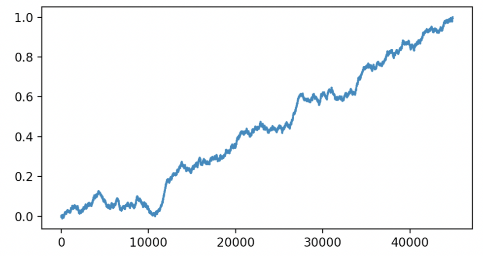
What is particularly interesting about this case is that, due the probability of change being slightly above \(50\%\), we can see that the sequence has an overall positive growth pattern; however, as far as daily returns is concerned, there is almost no value from day-to-day gains in the market.
To actually analyze the our expected value for the probability distributions in number of steps \(T\) to travel from \(0\) to \(1\), as a function of \(p, \epsilon\), we perform the following computation:
Expected Value of T
We set:
\begin{equation} \Delta = \begin{cases} +\epsilon, P=p\\ -\epsilon, P=1-p \end{cases} \end{equation}
Therefore, for \(T\) as a function from \(0\) to \(1\), we have:
\begin{align} E(T)&=\frac{1}{E\qty(\Delta) } \\ &= \frac{1}{p\epsilon-(1-p)\epsilon } \\ &= \frac{1}{\epsilon (2p-1)} \end{align}
Now we will calculate the Variance in \(T\):
\begin{align} Var(T) &= \frac{1}{Var(\Delta)} \end{align}
Where, \(Var(\Delta)\) is calculated by:
\begin{align} Var(\Delta) &= E(\Delta^{2})-E^{2}(\Delta) \\ &= \qty(\epsilon^{2} (2p-1)) - \qty(\epsilon (2p-1))^{2} \end{align}
And therefore:
\begin{equation} Var(T) = \frac{1}{\qty(\epsilon^{2} (2p-1)) - \qty(\epsilon (2p-1))^{2}} \end{equation}
Problem 3
Yes, as we expect, that as \(\epsilon\) decreases, the actual steps \(T\) it takes to travel from \([0,1]\) increases by an order of magnitude. Given \(10\) trials, with \(p=0.51\) and \(\epsilon = \{0.1,0.01\}\), we have that:
| \(\epsilon\) | Mean \(T\) | Std. \(T\) |
|---|---|---|
| 0.1 | 570.8 | 1051.142 |
| 0.01 | 3848.2 | 1457.180 |
We can see this on the expected value calculations as well, that:
\begin{equation} \lim_{\epsilon \to 0} E(T) = \frac{1}{\epsilon (2p-1)} = \infty \end{equation}
This is not true for the case of \(p=0.5\), where the limit will create an undefined behavior with \(0\infty\), and l’hospital’s rule upon \(\epsilon\) doesn’t apply here.
Problem 4
Yes, the quadratic variation converges towards \(0\). Similarly as before, with \(p=0.51\) and \(\epsilon = \{0.1,0.01,0.001\}\), our quadratic variations are:
| \(\epsilon\) | quadratic variation |
|---|---|
| 0.1 | 5.02 |
| 0.01 | 0.32 |
| 0.001 | 0.05 |
It seems like that, as long as the path terminates and epsilon becomes smaller, the sum of squared difference will converge towards \(0\).
This means that, for all \(p>0.5\), the squared differences will be convergent. However, for \(p\leq 0.5\), the squared differences are arguably still convergent but the sequence doesn’t terminate.
Problem 5
To allow negative values, we changed the function to:
\begin{equation} f(x) = ({x}-1)^{2} \end{equation}
The results of running the three expressions with \(p=0.51\), \(\epsilon=\{0.1, 0.01, 0.001\}\), similarly to before, respectively are as follows:
| \(\epsilon\) | \(f(x_{i})\) | \(f(x_{i+1})\) | \(f\qty(\frac{x_{i+1}-x_{i}}{2})\) |
|---|---|---|---|
| 0.1 | 3.03 | -2.37 | -1.85 |
| 0.01 | 1.7 | -1 | -0.17 |
| 0.001 | 0.359 | 0.307 | 0.938 |
It seems like—while all three of these results converge—they converge to distinctly different limits. Of course, this result also depends on \(p\), as the probability determines whether the path is even complete in the first place, which will of course affect the convergence here.