Let \(X\) denote price and \(Y\) denote volatility. The two objects obey the following process:
\begin{equation} \begin{cases} \dd{X} = \mu X \dd{t} + XY \dd{W} \\ \dd{Y} = \sigma Y \dd{B} \end{cases} \end{equation}
where, \(W\) and \(B\) are correlated Brownian motions with correlation \(\rho\) — \(E[(\dd{W})(\dd{B})] = \rho \dd{t}\).
Let’s work with \(Y\) first. We understand that \(Y\) is some continuous variable \(e^{a}\). Therefore, \(\dv{Y}{t}=ae^{a}\). Therefore, \(dY = ae^{a}dt\). Finally, then \(\frac{\dd{Y}}{Y} = \frac{ae^{a}}{e^{a}}\dd{t} = a\).
Finally, then, because we defined \(Y=e^{a} \implies \ln Y = a = \frac{\dd{Y}}{Y}\).
So, we have that:
\begin{align} &\dd{Y} = \sigma Y\dd{B} \\ \Rightarrow\ & \dd{\log Y} = \frac{\sigma Y\dd{B}}{Y} = \sigma \dd{B} \end{align}
This tells that the change in log returns in \(Y\) is normal (as \(B\) is a Brownian Motion), with a standard deviation of \(\sigma\). Therefore:
\begin{equation} \dd{\log Y} \sim \mathcal{N}(0, \sigma^{2} \dd{t}) \end{equation}
We therefore see that the log-returns of \(Y\) is a normal with variance \(\sigma^{2}\), making \(Y\) itself a Brownian Motion with center \(0\) and variance \(\sigma^{2}\).
So now, tackling the expression above in \(X\), we will do the same exact thing as above and divide by \(X\):
\begin{equation} \dd{\log X} = \mu \dd{t} + Y\dd{W} \end{equation}
So we can see that \(X\) is a Geometric Brownian Motion as a sum of two random variables—its volatility is determined by \(Y\) with a time-drift \(\mu \dd{t}\).
We see that we are almost ready to have an analytical solution here, because the top expression is applying some function \(f=\log\) to a stochastic differential equation by time; however, the right side \(Y\) here is not quite a constant (it is itself a stochastic process), so we can’t simply apply an Itô Intergral and call it a day.
So instead, we will proceed to a Monte-Carlo simulation of the results to verify as much as we can.
We will begin by setting the sane values for variances—having \(0.1\%\) drift and \(1\%\) variance in variance, and the two Brownian motions being inverses of each other \(\rho = 0.5\).
mu = 0.001
sigma = 0.01
rho = 0.5

(mu,sigma,rho)
(0.001, 0.01, 0.5)
We will seed a standard Brownian motion; as the two random motions are covariate, we can use the value of one to generate another: therefore we will return both at once.
from numpy.random import normal
def dbdw():
    dB = normal()
    dW = dB + normal(0, (1-rho)**2)
    return (dB, dW)
dbdw()
(-1.0246010237177643, -1.281335746614678)
Excellent.
We will now simulate the system we were given:
\begin{equation} \begin{cases} \dd{X} = \mu X \dd{t} + XY \dd{W} \\ \dd{Y} = \sigma Y \dd{B} \end{cases} \end{equation}
Let’s set the number of trials to \(10000\).
N = 1000
We will measure the convergence of \(\bar{\dd{X}}\) and \(\bar{\dd{Y}}\): we will tally each value at each time \(t\) as well as compare their expected values over time.
We will first seed our systems at \(1\%\) variance and \(1\) dollar of price.
X = 1
Y = 0.01
Now, it’s actual simulation time!
# history of Y and X
X_hist = []
Y_hist = []

# history of dx
dX_hist = []
dY_hist = []

# current expected value
EdX = 0
EdY = 0

# difference in E
EdX_diff = 0
EdY_diff = 0

# for n loops, we simulate
for _ in range(N):
    # get a source of randmess
    dB, dW = dbdw()

    # get the current dx and dw
    _dX = mu*X+X*Y*dW
    _dY = sigma*Y*dB

    # apply it
    X += _dX
    Y += _dY

    # tally it
    Y_hist.append(Y)
    X_hist.append(X)

    dX_hist.append(_dX)
    dY_hist.append(_dY)

    # calculate new expected value
    # we don't store it immediately b/c we want to check convergence
    _EdX = sum(dX_hist)/len(dX_hist)
    _EdY = sum(dY_hist)/len(dY_hist)

    EdX_diff = abs(_EdX-EdX)
    EdY_diff = abs(_EdY-EdY)

    # store new expected value
    EdX = _EdX
    EdY = _EdY
Let’s observe a few values! For starters, let’s measure our new expected values.
EdX
0.0013333651336800837
EdY
-1.225482645599256e-06
And, let’s check if we have converged by seeing if the difference is a reasonably small value:
(EdX_diff, EdY_diff)
(2.578663659035343e-05, 1.2183875816528115e-07)
Looks like both of our variables have converged. Now, let’s plot a few things. Let’s first build a table with our data.
import pandas as pd
data = pd.DataFrame({"price": X_hist, "variance": Y_hist})
data["time"] = data.index
data
        price  variance  time
0    0.998644  0.009974     0
1    0.980393  0.009796     1
2    0.998355  0.009967     2
3    0.994514  0.009913     3
4    1.001363  0.009961     4
..        ...       ...   ...
995  2.323640  0.008778   995
996  2.321473  0.008715   996
997  2.343427  0.008818   997
998  2.306271  0.008654   998
999  2.333365  0.008775   999

[1000 rows x 3 columns]
We will use this to continue the rest of our analysis. For data augmentation, we will also calculate the natural logs of the change to get the rate of change.
import numpy as np
data["price_log"] = np.log(data.price)
data["variance_log"] = np.log(data.variance)

data["price_log_change"] = data.price_log - data.price_log.shift(1)
data["variance_log_change"] = data.variance_log - data.variance_log.shift(1)

# drop the first row we have w/o change
data = data.dropna()
data
        price  variance  ...  price_log_change  variance_log_change
1    0.980393  0.009796  ...         -0.018444            -0.018005
2    0.998355  0.009967  ...          0.018155             0.017332
3    0.994514  0.009913  ...         -0.003855            -0.005443
4    1.001363  0.009961  ...          0.006863             0.004801
5    0.991306  0.009895  ...         -0.010094            -0.006639
..        ...       ...  ...               ...                  ...
995  2.323640  0.008778  ...          0.002148             0.002124
996  2.321473  0.008715  ...         -0.000933            -0.007227
997  2.343427  0.008818  ...          0.009413             0.011765
998  2.306271  0.008654  ...         -0.015983            -0.018804
999  2.333365  0.008775  ...          0.011680             0.013827

[999 rows x 7 columns]
Let’s begin by plotting what we have:
import seaborn as sns
import matplotlib.pyplot as plt

sns.set()
We will plot price and variation on two axes.
plt.gcf().clear()
sns.lineplot(x=data.time, y=data.price, color="g")
ax2 = plt.twinx()
sns.lineplot(x=data.time, y=data.variance, color="b", ax=ax2)
plt.show()
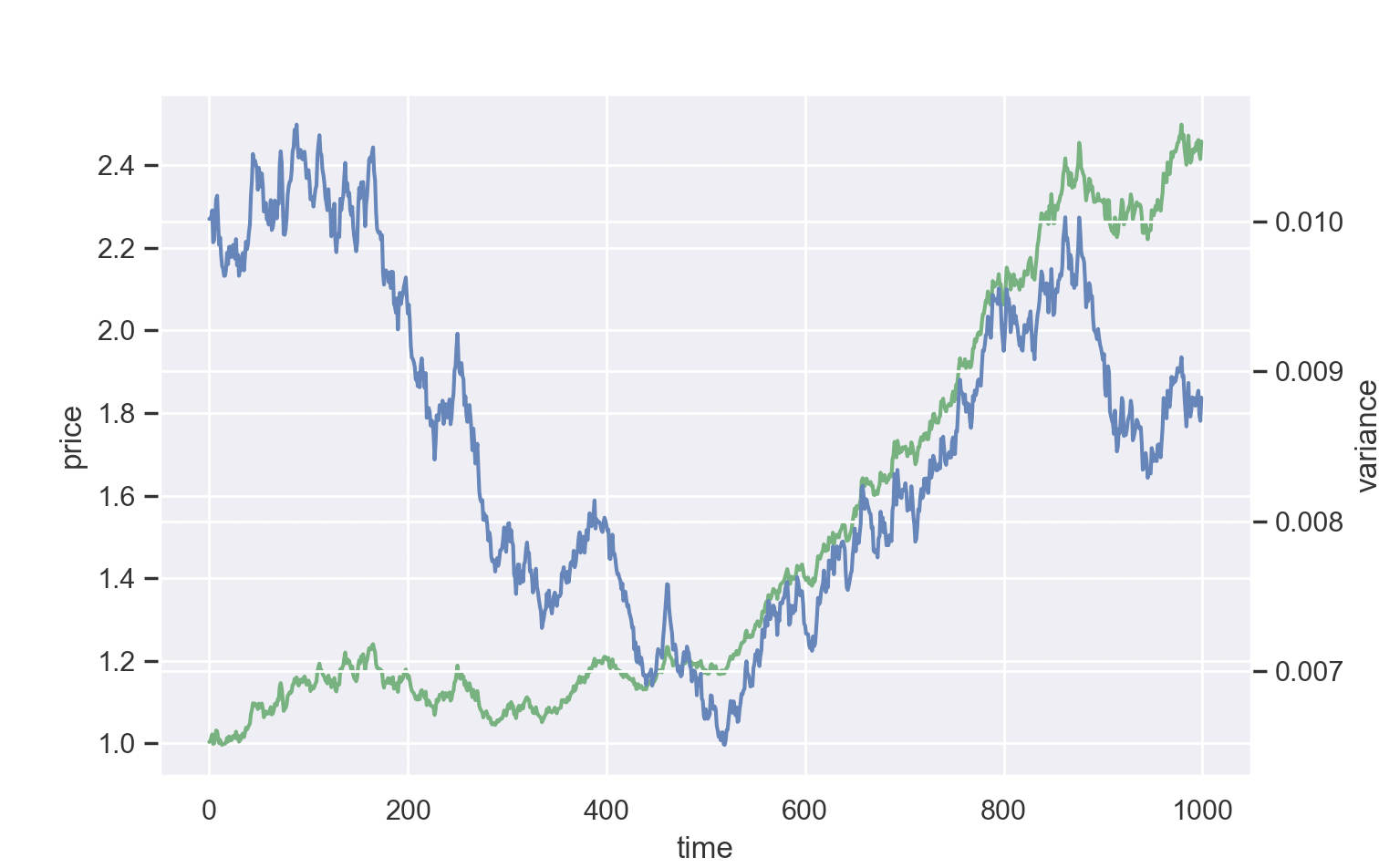
Where, the blue line represents the percent variance over time and the green line represents the price. Given the \(0.1\%\) drift we provided, we can see that our simulated market grows steadily in the 1000 data point.
We can then plot the log (percent) changes.
plt.gcf().clear()
sns.lineplot(x=data.time, y=data.price_log_change, color="g")
ax2 = plt.twinx()
sns.lineplot(x=data.time, y=data.variance_log_change, color="b", ax=ax2)
plt.show()
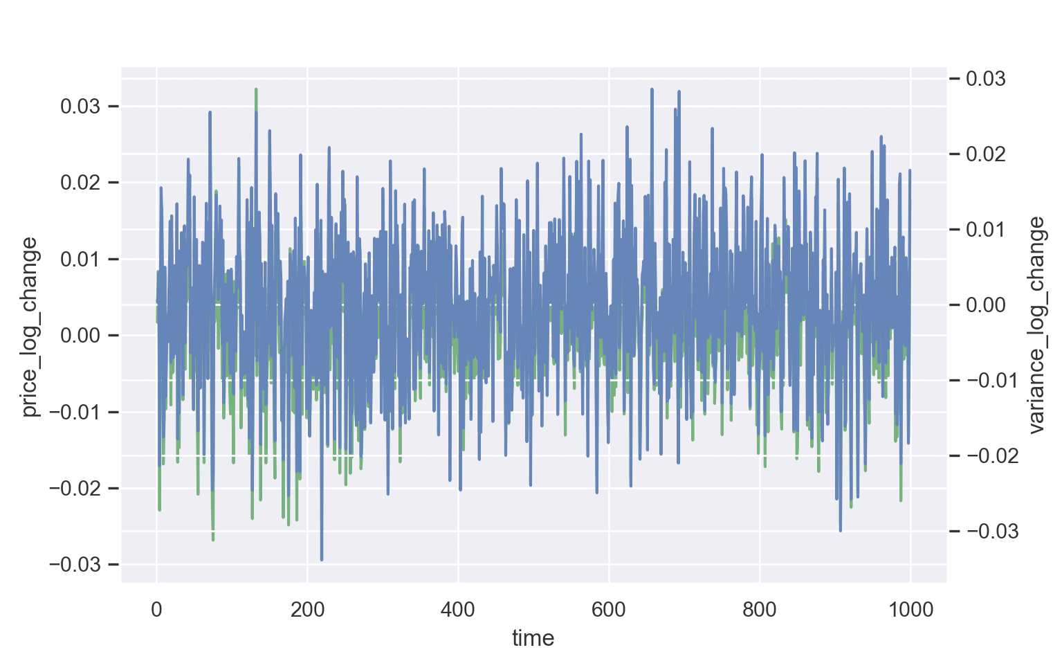
As you can see—we have fairly strong random variables, centered around \(0\). Having verified that our drift and variables behave in the way that we expect, we can proceed with analysis.
We can use a single-variable \(t\) test to figure the \(99\%\) confidence band of the result. To do this, we first need to calculate the mean and standardized deviation of the price percent change (log difference).
log_mean, log_std = (data.price_log_change.mean(), data.price_log_change.std())
(log_mean, log_std)
(0.0008495184126335735, 0.008471735971085885)
And now, we will calculate the
from scipy.stats import t
lower_bound, upper_bound = t.interval(0.99, len(data)-1, loc=log_mean, scale=log_std)
lower_bound
-0.021014037766751738
Therefore, with \(99\%\) confidence, we can say that our asset—given its current parameters, and an \(N=1000\) Monte-Carlo simulation—will not have a more than \(2.1\%\) drop in value.
We will use a hedged option to minimize loss. We will use this value to determine the maximum loss for an European put option, maturing in \(T\) time, such that the exercise thereof will be hedged against drops of asset price.
First, we will determine the cost of a correctly hedged European put option.
We will define \(S_{0}\) as the current price of the asset. We will use \(P\) as the price of the put option.
We desire the strike price of the option to be:
\begin{equation} K = S_{0} + P \end{equation}
that is: the price of the put option we desire here will recuperate the price to trade the option and protect against loss. We will symbolically solve for the price of such an option.
Note that the codeblocks switches here from standard Python to SageMath.
We first define the standard normal cumulative distribution.
from sage.symbolic.integration.integral import definite_integral
z = var("z")
N(x) = 1/sqrt(2*pi)*definite_integral(e^(-z^2/2), z, -infinity, x)
We will then leverage the Euopean call Black-Scholes model to calculate the optimal put price. We first instantiate variables \(T\), and we will set current time to be \(0\).
We will use \(v\) for \(\sigma\), the volatility of the security. We will use \(S\) for current price. Lastly, we define \(P\) to be our put price. We will call \(r\) our risk-free rate.
To determine the discount factor, we first implement symbolically our expression for desired strike price.
v,T,S,P,r = var("v T S P r")
K = S+P
K
P + S
Great. Now we will implement our discount factors.
d1 = 1/v*sqrt(T) * (ln(S/K) + (r+v^2/2)*(T))
d2 = d1-v*T
d1, d2
(1/2*((v^2 + 2*r)*T + 2*log(S/(P + S)))*sqrt(T)/v,
 -T*v + 1/2*((v^2 + 2*r)*T + 2*log(S/(P + S)))*sqrt(T)/v)
And lastly, we will implement the Black-Scholes expression for puts as a logical expression.
expr = P == N(-d2)*K*e^(-r*T)-N(-d1)*S
expr
\begin{equation} P = \frac{{\left({\left(\operatorname{erf}\left(\frac{\sqrt{2} {\left(T v^{2} + 2 \, T r + 2 \, \log\left(\frac{S}{P + S}\right)\right)} \sqrt{T}}{4 \, v}\right) - 1\right)} e^{\left(T r\right)} - \operatorname{erf}\left(-\frac{\sqrt{2} {\left(2 \, T v^{2} - {\left(T v^{2} + 2 \, T r + 2 \, \log\left(\frac{S}{P + S}\right)\right)} \sqrt{T}\right)}}{4 \, v}\right) + 1\right)} S}{\operatorname{erf}\left(-\frac{\sqrt{2} {\left(2 \, T v^{2} - {\left(T v^{2} + 2 \, T r + 2 \, \log\left(\frac{S}{P + S}\right)\right)} \sqrt{T}\right)}}{4 \, v}\right) + 2 \, e^{\left(T r\right)} - 1} \end{equation}
Numerical solutions to this expression—fitting for each of the values from before—would then indicate the correct price of the option to generate the hedging effect desired.