Two steps:
- obtaining a function for the gradient of policy against some parameters \(\theta\)
- making them more based than they are right now by optimization
Thoughout all of this, \(U(\theta)\) is \(U(\pi_{\theta})\).
Obtaining a policy gradient
Finite-Difference Gradient Estimation
We want some expression for:
\begin{equation} \nabla U(\theta) = \qty[\pdv{U}{\theta_{1}} (\theta), \dots, \pdv{U}{\theta_{n}}] \end{equation}
we can estimate that with the finite-difference “epsilon trick”:
\begin{equation} \nabla U(\theta) = \qty[ \frac{U(\theta + \delta e^{1}) - U(\theta)}{\delta} , \dots, \frac{U(\theta + \delta e^{n}) - U(\theta)}{\delta} ] \end{equation}
where \(e^{j}\) is the standard basis vector at position \(j\). We essentially add a small \(\delta\) to the \(j\) th slot of each parameter \(\theta_{j}\), and divide to get an estimate of the gradient.
Linear Regression Gradient Estimate
We perform \(m\) random perturbations of \(\theta\) parameters, and lay each resulting parameter vector flat onto a matrix:
\begin{equation} \Delta \theta = \mqty[(\Delta \theta^{1})^{T} \\ \dots \\ (\Delta \theta^{m})^{T}] \end{equation}
For \(\theta\) that contains \(n\) parameters, this is a matrix \(m\times n\).
We can now write out the \(\Delta U\) with:
\begin{equation} \Delta U = \qty[U(\theta+ \Delta \theta^{1}) - U(\theta), \dots, U(\theta+ \Delta \theta^{m}) - U(\theta)] \end{equation}
We have to compute Roll-out utility for each \(U(\theta + …)\)
We now want to fit a function between \(\Delta \theta\) to \(\Delta U\), because from the definition of the gradient we have:
\begin{equation} \Delta U = \nabla_{\theta} U(\theta)\ \Delta \theta \end{equation}
(that is \(y = mx\))
Rearranging the expression above
\begin{equation} \nabla_{\theta} U(\theta) \approx \Delta \theta^{\dagger} \Delta U \end{equation}
where \(\Delta \theta^{\dagger}\) is the pseudoinverse of \(\Delta \theta\) matrix.
To end up at a gradient estimate.
Likelyhood Ratio Gradient
This is likely good, but requires a few things:
- an explicit transition model that you can compute over
- you being able to take the gradient of the policy
this is what people usually refers to as “Policy Gradient”.
Recall:
\begin{align} U(\pi_{\theta}) &= \mathbb{E}[R(\tau)] \\ &= \int_{\tau} p_{\pi} (\tau) R(\tau) d\tau \end{align}
Now consider:
\begin{align} \nabla_{\theta} U(\theta) &= \int_{\tau} \nabla_{\theta} p_{\pi}(\tau) R(\tau) d \tau \\ &= \int_{\tau} \frac{p_{\pi} (\tau)}{p_{\pi} (\tau)} \nabla_{\tau} p_{\tau}(\tau) R(\tau) d \tau \end{align}
Aside 1:
Now, consider the expression:
\begin{equation} \nabla \log p_{\pi} (\tau) = \frac{\nabla p_{\pi}(\tau)}{p_{\pi} \tau} \end{equation}
This is just out of calculus. Consider the derivative chain rule; now, the derivative of \(\log (x) = \frac{1}{x}\) , and the derivative of the inside is \(\nabla x\).
Rearranging that, we have:
\begin{equation} \nabla p_{\pi}(\tau) = (\nabla \log p_{\pi} (\tau))(p_{\pi} \tau) \end{equation}
Substituting that in, one of our \(p_{\pi}(\tau)\) cancels out, and, we have:
\begin{equation} \int_{\tau} p_{\pi}(\tau) \nabla_{\theta} \log p_{\pi}(\tau) R(\tau) \dd{\tau} \end{equation}
You will note that this is the definition of the expectation of the right half (everything to the right of \(\nabla_{\theta}\)) vis a vi all \(\tau\) (multiplying it by \(p(\tau)\)). Therefore:
\begin{equation} \nabla_{\theta} U(\theta) = \mathbb{E}_{\tau} [\nabla_{\theta} \log p_{\pi}(\tau) R(\tau)] \end{equation}
Aside 2:
Recall that \(\tau\) a trajectory is a pair of \(s_1, a_1, …, s_{n}, a_{d}\).
We want to come up with some \(p_{\pi}(\tau)\), “what’s the probability of a trajectory happening given a policy”.
\begin{equation} p_{\pi}(\tau) = p(s^{1}) \prod_{k=1}^{d} p(s^{k+1} | s^{k}, a^{k}) \pi_{\theta} (a^{k}|s^{k}) \end{equation}
(“probably of being at a state, times probability of the transition happening, times the probability of the action happening, so on, so on”)
Now, taking the log of it causes the product to become a summation:
\begin{equation} \log p_{\pi}(\tau) = p(s^{1}) + \sum_{k=1}^{d} p(s^{k+1} | s^{k}, a^{k}) + \pi_{\theta} (a^{k}|s^{k}) \end{equation}
Plugging this into our expectation equation:
\begin{equation} \nabla_{\theta} U(\theta) = \mathbb{E}_{\tau} \qty[\nabla_{\theta} \qty(p(s^{1}) + \sum_{k=1}^{d} p(s^{k+1} | s^{k}, a^{k}) + \pi_{\theta} (a^{k}|s^{k})) R(\tau)] \end{equation}
This is an important result. You will note that \(p(s^{1})\) and \(p(s^{k+1}|s^{k},a^{k})\) doesn’t have a \(\theta\) term in them!!!!. Therefore, taking term in them!!!!*. Therefore, taking the \(\nabla_{\theta}\) of them becomes… ZERO!!! Therefore:
\begin{equation} \nabla_{\theta} U(\theta) = \mathbb{E}_{\tau} \qty[\qty(0 + \sum_{k=1}^{d} 0 + \nabla_{\theta} \pi_{\theta} (a^{k}|s^{k})) R(\tau)] \end{equation}
So based. We now have:
\begin{equation} \nabla_{\theta} U(\theta) = \mathbb{E}_{\tau} \qty[\sum_{k=1}^{d} \nabla_{\theta} \log \pi_{\theta}(a^{k}|s^{k}) R(\tau)] \end{equation}
where,
\begin{equation} R(\tau) = \sum_{k=1}^{d} r_{k}\ \gamma^{k-1} \end{equation}
“this is very nice” because we do not need to know anything regarding the transition model. This means we don’t actually need to know what \(p(s^{k+1}|s^{k}a^{k})\) because that term just dropped out of the gradient.
We can simulate a few trajectories; calculate the gradient, and average them to end up with our overall gradient.
Reward-to-Go
Variance typically increases with Rollout depth. We don’t want that. We want to correct for the causality of action/reward. Action in the FUTURE do not influence reward in the PAST.
Recall:
\begin{equation} R(\tau) = \sum_{k=1}^{d} r_{k}\ \gamma^{k-1} \end{equation}
Let us plug this into the policy gradient expression:
\begin{equation} \nabla_{\theta} U(\theta) = \mathbb{E}_{\tau} \qty[\sum_{k=1}^{d} \nabla_{\theta} \log \pi_{\theta}(a^{k}|s^{k}) \qty(\sum_{k=1}^{d} r_{k}\ \gamma^{k-1})] \end{equation}
Let us split this reward into two piece; one piece for the past (up to \(k-1\)), and one for the future:
\begin{equation} \nabla_{\theta} U(\theta) = \mathbb{E}_{\tau} \qty[\sum_{k=1}^{d} \nabla_{\theta} \log \pi_{\theta}(a^{k}|s^{k}) \qty(\sum_{l=1}^{k-1} r_{l}\ \gamma^{l-1} + \sum_{l=k}^{d} r_{l}\ \gamma^{l-1})] \end{equation}
We now want to ignore all the past rewards (i.e. the first half of the internal summation). Again, this is because action in the future shouldn’t care about what reward was gather in the past.
\begin{equation} \nabla_{\theta} U(\theta) = \mathbb{E}_{\tau} \qty[\sum_{k=1}^{d} \nabla_{\theta} \log \pi_{\theta}(a^{k}|s^{k}) \sum_{l=k}^{d} r_{l}\ \gamma^{l-1}] \end{equation}
We now factor out \(\gamma^{k-1}\) to make the expression look like:
\begin{equation} \nabla_{\theta} U(\theta) = \mathbb{E}_{\tau} \qty[\sum_{k=1}^{d} \nabla_{\theta} \log \pi_{\theta}(a^{k}|s^{k}) \qty(\gamma^{k-1} \sum_{l=k}^{d} r_{l}\ \gamma^{l-k})] \end{equation}
We call the right term Reward-to-Go:
\begin{equation} r_{togo}(k) = \sum_{l=k}^{d} r_{l}\ \gamma^{l-k} \end{equation}
where \(d\) is the depth of your trajectory and \(k\) is your current state. Finally, then:
\begin{equation} \nabla_{\theta} U(\theta) = \mathbb{E}_{\tau} \qty[\sum_{k=1}^{d} \nabla_{\theta} \log \pi_{\theta}(a^{k}|s^{k}) \qty(\gamma^{k-1} r_{togo}(k))] \end{equation}
Baseline subtraction
Sometimes, we want to subtract a baseline reward to show how much actually better an action is (instead of blindly summing all future rewards). This could be the average reward at all actions at that state, this could be any other thing of your choosing.
\begin{equation} \nabla_{\theta} U(\theta) = \mathbb{E}_{\tau} \qty[\sum_{k=1}^{d} \nabla_{\theta} \log \pi_{\theta}(a^{k}|s^{k}) \qty(\gamma^{k-1} (r_{togo}(k) - r_{baseline}(k)))] \end{equation}
For instance, if you have a system where each action all gave \(+1000\) reward, taking any particular action isn’t actually very good. Hence:
Optimizing the Policy Gradient
We want to make \(U(\theta)\) real big. We have two knobs: what is our objective function, and what is your restriction?
Policy Gradient Ascent
good ‘ol fashioned
\begin{equation} \theta \leftarrow \theta + \alpha \nabla U(\theta) \end{equation}
where \(\alpha\) is learning rate/step factor. This is not your STEP SIZE. If you want to specify a step size, see Restricted Step Method.
Restricted Step Method
Policy Gradient Ascent can take very large steps if the gradient is too large.
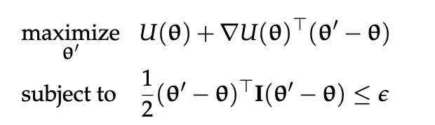
One by which we can optimize the gradient, ensuring that we don’t take steps larger than:
\begin{equation} \frac{1}{2}(\theta’ - \theta)^{T} I(\theta’ - \theta) \leq \epsilon \end{equation}
is through Restricted Gradient:
\begin{equation} \theta \leftarrow \theta + \sqrt{2 \epsilon} \frac{\nabla U(\theta)}{|| \nabla U(\theta)||} \end{equation}
Occasionally, if a step-size is directly given to you in terms of euclidean distance, then you would replace the entirety of \(\sqrt{2 \epsilon}\) with your provided step size.
Trust Region Policy Optimization
Using a different way of restricting the update.
Proximal Policy Optimization
Clipping the gradients.