probability distribution

probability distributions “assigns probability to outcomes”

\(X\) follows distribution \(D\). \(X\) is a “\(D\) random variable”, where \(D\) is some distribution (normal, gaussian, etc.)

syntax: \(X \sim D\).

Each distribution has three properties:

variables (what is being modeled)
values (what values can they take on)
parameters (how many degrees of freedom do we have)

Types of Distribution

parametrized distribution

We often represent probability distribution using a set of parameters \(\theta_{j}\). For instance, a normal distribution is given by \(\mu\) and \(\sigma\), and a PMF is by the probability mass for each.

Methods of Compressing the Parameters of a Distribution

So, for instance, for a binary distribution with \(n\) variables which we know nothing about, we have:

\begin{equation} 2^{n} - 1 \end{equation}

parameters (\(2^{n}\) different possibilities of combinations, and \(1\) non-free variables to ensure that the distribution add up)

assuming independence

HOWEVER, if the variables were independent, this becomes much easier. Because the variables are independent, we can claim that:

\begin{equation} p(x_{1\dots n}) = \prod_{i}^{} p(x_{i)) \end{equation}

decision tree

For instance, you can have a decision tree which you selectively ignore some combinations.

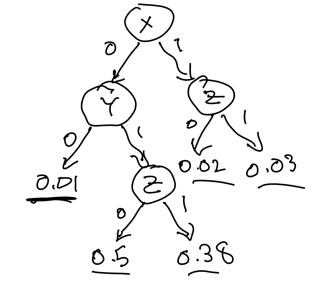
In this case, we ignored \(z\) if both \(x\) and \(y\) are \(0\).

Baysian networks

see Baysian Network

types of probability distributions

distribution of note

uniform distribution
gaussian distributions

uniform distribution

\begin{equation} X \sim Uni(\alpha, \beta) \end{equation}

\begin{equation} f(x) = \begin{cases} \frac{1}{\beta -\alpha }, 0\leq x \leq 10 \\0 \end{cases} \end{equation}

\begin{equation} E[x] = \frac{1}{2}(\alpha +\beta) \end{equation}

\begin{equation} Var(X) = \frac{1}{12}(\beta -\alpha )^{2} \end{equation}

Gaussian Things

Truncated Gaussian distribution

Sometimes, we don’t want to use a Gaussian distribution for values above or below a threshold (say if they are physically impossible). In those cases, we have some:

\begin{equation} X \sim N(\mu, \sigma^{2}, a, b) \end{equation}

bounded within the interval of \((a,b)\). The PDF of this function is given by:

\begin{equation} N(\mu, \sigma^{2}, a, b) = \frac{\frac{1}{\sigma} \phi \qty(\frac{x-\mu }{\sigma })}{\Phi \qty(\frac{b-\mu }{\sigma }) - \Phi \qty(\frac{a-\mu}{\sigma})} \end{equation}

where:

\begin{equation} \Phi = \int_{-\infty}^{x} \phi (x’) \dd{x’} \end{equation}

and where \(\phi\) is the standard normal density function.

three ways of analysis

cumulative distribution function

What is the probability that a random variable takes on value less tha

\begin{equation} cdf_{x}(x) = P(X<x) = \int_{-\infty}^{x} p(x’) dx' \end{equation}

sometimes written as:

\begin{equation} F(x) = P(X < x) \end{equation}

Recall that, with

quantile function

\begin{equation} \text{quantile}_{X}(\alpha) \end{equation}

is the value \(x\) such that:

\begin{equation} P(X \leq x) = \alpha \end{equation}

That is, the quantile function returns the minimum value of \(x\) at which point a certain cumulative distribution value desired is achieved.

adding uniform distribution

for \(1 < a < 2\)

\begin{equation} f(X+Y = a) = \begin{cases} a, 0 < a < 1, \\ 2-a, 1 < a < 2, \\ 0, otherwise \end{cases} \end{equation}