Each query presents one item and records a binary response (did they like it?).
- Rasch: a person parameter \(\alpha\)
- Frozen encoder: reward-heads weights \(w\)
We don’t want to present too many queries to train this.
Fisher Information
Fisher recognizes fixed \(u\), and have expectation under different measures Y
New User, Known Object
Suppose you want to know the information gain from understanding \(\alpha\) the user parameter, conditioned on some known item you tested \(\beta\). Consider some random variable \(Y\) under some kind of Rasch model:
\begin{equation} Y | \alpha, \beta \sim \text{Bern}\qty(p), p = \sigma\qty(\alpha - \beta) \end{equation}
where \(Y=1\) denotes a correct response. Write: \(\ell\qty(\alpha, y, \beta) = \log P\qty(Y=y \mid \alpha, \beta)\); the Fisher information is:
\begin{equation} \mathcal{I}\qty(\alpha; \beta) = \mathbb{E}\qty [\qty(\dv{l}{\alpha})^{2} \mid\alpha, \beta] \end{equation}
And you can get \(P\qty(Y=y)\) from standard Bernouli situation. If you write this out, you will get:
\begin{equation} \mathcal{I}\qty(\alpha; \beta) = \mathbb{E}\qty(Y - p)^{2} \mid \alpha , \beta \end{equation}
And now, since random variable \(Y\) takes on \(1\) with probability \(p\), and takes on \(0\) with proabbility \(1-p\), then this gives:
\begin{equation} \mathcal{I}\qty(\alpha; \beta) = \mathbb{E}\qty(Y - p)^{2} = p\qty(1-p)^{2} + \qty(1-p) \qty(-p)^{2} = p\qty(1-p) \end{equation}
Now Factor Models
I don’t quite get this
For each query, write:
\begin{equation} \Lambda_{v} = \Lambda + \mathcal{I} \qty(v; \hat{u}) \end{equation}
where you write \(\sigma\qty(\alpha-\beta)\) in terms of \(\hat{U}^{T} V\) instead. There’s a few different types of way to design \(\Lambda_{v}\)
| Criteria | Goal | Local Covariance |
|---|---|---|
| A-optimal | min \(tr\qty(\Lambda_{v}^{-1})\) | reduce sum of covariance |
| D-optimal | max \(\log \det (\Delta_{v})\) | reduce the volume of an uncertainty |
| E-optimal | max \(\lambda_{\min}\) | recudec small eigenvalue |
Consider D-optimal design.
\begin{equation} \Delta_{d}\qty(u) = \log \qty(1 + w_{v}u^{T}\Sigma u) \end{equation}
where \(\Sigma = \Delta^{-1}\), and \(w_{v} = \hat{p}_{u} \qty(1-\hat{p}_{u})\). Where we use factor model for \(p_{u} = \sigma\qty(u^{T}v + d)\). Fisher gives:
\begin{equation} I\qty(v; u) = p_{u}\qty(1-p_{u}) v v^{T} \end{equation}
Let’s define:
\begin{equation} \Lambda = \Lambda_{0} +\sum_{t=1}^{n} \hat{p}_{t}\qty(1-\hat{p}_{t}) v_{t}v_{t}^{T} \end{equation}
Mutual Information
Consider you measured some data \(D\) of user \(u\) against document \(Y\). Perhaps we want to some kind of prior about the user, but unlike before we are not super sure about the point estimate.
\begin{equation} I\qty(u; Y|D,v,d) = \mathbb{E}_{u,Y | D, v, d} \qty [\log \frac{p\qty(u,Y | D, v, d)}{p\qty(u | D) p\qty(Y|D, v,d)}] \end{equation}
We call this the “expected information gain”, since
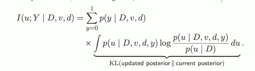
Similarly, by applying Bayes rule, we can get:
\begin{equation} \text{EIG}\qty(v,d) = H\qty(Y|D,v,d) - \mathbb{E}_{u | D}\qty [H\qty(Y| u,v,d)] \end{equation}
where: \(H\qty(Y) = - \mathbb{E}_{Y}\qty [\log p\qty(Y)]\).
Computing information gain
Give draws \(p_{m} = \sigma \qty(\qty(u^{(m)})^{T} v + d)\), \(p_{m} = \frac{1}{M} \sum_{m=1}^{M} p_{m}\) and \(M\) data points. Consider:
\begin{equation} \text{EIG}\qty(v,d) = h\qty(p_{M})- \frac{1}{M}\sum_{m=1}^{M} h\qty(p_{m}) \end{equation}
For neural head
\begin{equation} r_{w}\qty(x, a) = w^{T}h_{\phi}\qty(x,a) \end{equation}
for context \(x\) and item \(a\). Consider:
\begin{equation} P\qty(Y = 1 \mid u,v, d) = \sigma \qty(u^{T} v + d) \end{equation}
we can estimate \(p\qty(u|D)\) by pprior \(u \sim \mathcal{N}\qty(u, \Sigma)\).
\begin{equation} Z = u^{T} v + d \sim \mathcal{N}\qty(u_{v}, s^{2}_{v}), u_{v} = u^{T} v +d, s_{v}^{2} = u^{T}\Sigma v \end{equation}
Example
Consider posterior:
\begin{equation} u \sim \mathcal{N}\qty(0,1) \end{equation}
and known offset \(d = 0\). Suppose you had two items with encodings: \(v_{A} = 0.25\), \(v_{B} = 2\). We have: