Most users are incapable of writing good Boolean Retrieval queries.
feast or famine problem
Boolean Retrieval either returns too few or too many results: AND queries return often too few results \(\min (x,y)\), and OR queries return too many results \(x+y\).
This is not a problem with Ranked Information Retrieval because a large result set doesn’t matter: top results just needs to be good results.
free text query
Instead of using a series of Boolean Retrieval, we instead give free text to the user.
score
To do Ranked Information Retrieval, we need a way of asigning a score to a query-document pair.
- the more frequently the query term appears in the doc, the higher the score should be
- if the word doesn’t appear, we score as 0
Jaccard Coefficient
\begin{equation} jaccard(A,B) = |A \cap B | / |A \cup B| \end{equation}
where \(A\) and \(B\) are vocab, (i.e. no frequency).
limitation
- doesn’t consider frequency
- rare terms are more informative than frequent terms
- the normalization isn’t quite right, ideally we should use \(\sqrt{A\cup B}\), which can be obtained via cosine-similarity
log-frequency weighting
“Relevance does not increase proportionally with term frequency”—a document with 10 occurrences of a term is more relevant than that with 1, but its not 10 times more relevant.
\begin{equation} w_{t,d} = \begin{cases} 1 + \log_{10} (tf_{t,d}), \text{if } tf_{t,d} > 0 \\ 0 \end{cases} \end{equation}
this gives less-than-linear growth.
to score, we add up all the terms which intersect.
document frequency
the document frequency is the number of documents in which a term occur.
Its an INVERSE MEASURE of the informativeness of a word—the more times a word appears, the less informative it is.
\begin{equation} idf_{t} = \log_{10} (N / df_{t}) \end{equation}
where \(N\) is the number of documents, and \(df_{t}\) is the number of documents in which the term appears. We take the log in the motivation as log-frequency weighting.
“a word that occurs in every document has a weight of \(0\)”.
There is no effect to one-term queries.
We don’t use collection frequencies (i.e. we never consider COUNTS in CORPUS, because collection frequencies would score commonly found words equally because it doesn’t consider distribution).
TF-IDF
multiply log-frequency weighting TIMES document frequency.
\begin{equation} score(q,d) = \sum_{t \in q \cap d} (1+\log_{10}(tf_{t,d})) \times \log_{10}\qty(\frac{N}{df_{t}}) \end{equation}
if \(tf = 0\), set the entire TF score to \(0\) without adding 1.
using this, we can now construct a weight-matrix. Each document is a vector of the TFIDF score for each term against each document.
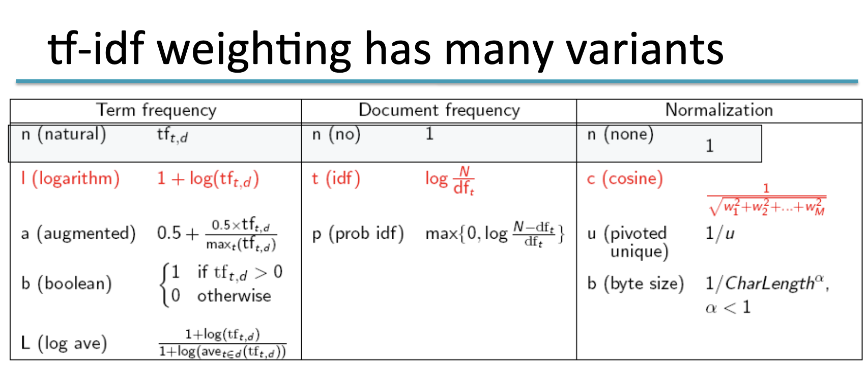
There are a series of approaches that you can use as a possible approach to compute tfidf: various ways to normalizing, variable document frequency counts (or not use it), etc.
SMART notation
ddd.qqq, where the first three letters represent the document weighting scheme, and the second three letter represents the query weighting scheme.
vector-space model
after creating a matrix where each column is a document and each row is a term, and the cells are TF-IDF of the words against the documents, we can consider each document as a vector over the team.
we can treat queries as ALSO a document in the space, and therefore use proximity of the vectors as a searching system.
(Euclidian distance is bad: because its too large for vectors of different lengths. Instead, we should use angle instead of distance.)
cosine similarity
\begin{equation} \cos(q,d) = \frac{q \cdot d}{|q| |d|} \end{equation}
because the dot product becomes just the angle between the two vectors after you normalize by length.
typically, you may want to normalize the length of the vectors in advance.
cosine is a little flatten ontop
ltc.lnn weighting
document: logarithm + idf + normed query: logarithm + 1 + 1
meaning, we don’t weight or normalize query vectors