We learn a Bayes Net grphical structure by following Bayes rule:
\begin{align} P(G|D) &\propto P(D|G) P(G) \\ &= P(G) \int P(D | \theta, G) P(\theta|G) d\theta \\ &= P(G) \prod_{i=1}^{n} \prod_{j=1}^{q_{i}} \frac{\Gamma(\alpha_{i,j,0})}{\Gamma(\alpha_{i,j,0} + m_{i,j,0})} \prod_{k=1}^{r_{i}} \frac{\Gamma(\alpha_{i,j,k} + m_{i,j,k})}{\Gamma(\alpha_{i,j,k})} \end{align}
where, we define: \(\alpha_{i,j,0} = \sum_{k} \alpha_{i,j,k}\).
The actual integration process is not provided, but mostly uninteresting. See Beta Distribution for a flavour of how it came about.
This is hard. We are multiply many gammas together, which is computationally lame. So instead, we use
Baysian Network Scoring
Log Bayesian Score is a score for measure of well-fittingness of a Baysian Network against some data. We sometimes call this the Baysian Score.
Let:
- \(x_{1:n}\) be variables
- \(o_1, …, o_{m}\) be the \(m\) observations we took
- \(G\) is the graph
- \(r_{i}\) is the number of instantiations in \(X_{i}\) (for boolean variables, this would be \(2\))
- \(q_{i}\) is the number of parental instantiations of \(X_{i}\) (if parent 1 can take on 10 values, parent 2 can take 3 values, then child’s \(q_{i}=10\cdot 3=30\)) — if a node has no parents it has a \(q_{i}\) is \(1\)
- \(\pi_{i,j}\) is \(j\) instantiation of parents of \(x_{i}\) (the \(j\) th combinator)
Let us first make some observations. We use \(m_{i,j,k}\) to denote the COUNT of the number of times \(x_{i}\) took a value \(k\) when \(x_{i}\) parents took instantiation \(j\).
We aim to compute:
\begin{equation} \log P(G|D) = \log P(G) + \sum_{i=1}^{n} \sum_{j=1}^{q_{i}} \qty[\qty(\log \frac{\Gamma(\alpha_{i,j,0})}{\Gamma(\alpha_{i,j,0}+ m_{i,j,0})}) + \sum_{k=1}^{r_{i}} \log \frac{\Gamma(\alpha_{i,j,k} + m_{i,j,k})}{\Gamma(\alpha_{i,j,k})}] \end{equation}
In practice, uniform prior of the graph is mostly used always. Assuming uniform priors, so \(P(G)=1\) and therefore we can drop the first term. Recall that \(\alpha_{i,j,0} = \sum_{k} \alpha_{i,j,k}\).
We can effectively take a prior structure, and blindly compute the Baysian Score vis a vi your data, and you will get an answer which whether or not something is the simplest model.
Of course, we can’t just try all graphs to get a graph structure. Instead, we use some search algorithm:
K2 Algorithm
Runs in polynomial time, but doesn’t grantee an optimal structure. Let us create a network with a sequence of variables with some ordering:
\begin{equation} x_1, x_2, x_3, x_4 \end{equation}
For K2 Algorithm, we assume a uniform distribution initially before the graph is learned.
- we lay down \(x_1\) onto the graph
- we then try to lay down \(x_{2}\): compute the Baysian Scores of two networks: \(x_1 \to x_2\) OR \(x_1\ x_2\) (see if connecting \(x_2\) to \(x_1\) helps). keep the structure with the maximum score
- we then try to lay down \(x_{3}\): compute the Baysian Score of \(x_1 \to x_3\) (plus whatever decision you made about \(x_2\)) OR \(x_1, x_3\); keep the one that works the best. Then, try the same to decide whether to connect \(x_2\) to \(x_3\) as well
- Repeat until you considered all nodes
After you try out one ordering, you should try out another one. Because you can only add parents from elements before you in the list, you will never get a cycle.
Local Graph Search
Start with an uncorrected graph. Search on the following actions:
- add edge
- remove edge
- flip edge
A graph’s neighborhood is the graphs for whicthey are one basic graph operation away.
Create a cycle detection scheme.
Now, just try crap. Keep computing a Baysian Score after you tried something, if its good, keep it. If its not, don’t.
To prevent you from being stuck in a local minimum:
- perform random restarts
- perform K2 Algorithm, and then try things out
- simulated annealing: take a step that’s worse for optimizing Baysian Scores
- genetic algorithms: random population which reproduces at a rate proportional to their score
Partially Directed Graph Search
We first formulate a partially-directed graph, which is a graph which has some edges, but some edges left to be decided:
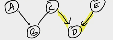
In this case, edges \(C \to D\) and \(D \leftarrow E\) are both defined. \(A,B,C\) are left as undirected nodes available to be searched on.
We now try out all combinations of arrows that may fit between \(A,B,C\), with the constraint of all objects you search on being Markov Equivalent (so, you can’t remove or introduce new immoral v-structures).