Neural Networks are powerful because of self organization of the intermediate levels.
Neural Network Layer
\begin{equation} z = Wx + b \end{equation}
for the output, and the activations:
\begin{equation} a = f(z) \end{equation}
where the activation function \(f\) is applied element-wise.
Why are NNs Non-Linear?
- there’s no representational power with multiple linear (though, there is better learning/convergence properties even with big linear networks!)
- most things are non-linear!
Activation Function
We want non-linear and non-threshold (0/1) activation functions because it has a slope—meaning we can perform gradient-based learning.
sigmoid
sigmoid: it pushed stuff to 1 or 0.
\begin{equation} \frac{1}{1+e^{-z}} \end{equation}
tanh
\begin{equation} tanh(z) = \frac{e^{z}-e^{-z}}{e^{z}+e^{-z}} \end{equation}
this is just rescaled logistic: its twice as steep (tanh(z) = 2sigmoid(2z)-1)
hard tanh
tanh but funny. because exp is hard to compute
\begin{equation} HTanh = \begin{cases} -1, if x < -1 \\ 0, if -1 \leq x \leq 1 \\ 1, if x > 1\\ \end{cases} \end{equation}
this motivates ReLU
relu
slope is 1 so its easy to compute, etc.
\begin{equation} ReLU(z) = \max(z,0) \end{equation}
Leaky ReLU
“ReLU like but not actually dead”
\begin{equation} LeakReLU = \begin{cases} x, if x>0 \\ \epsilon x, if x < 0 \end{cases} \end{equation}
or slightly more funny ones
\begin{equation} swish = x \sigma(x) \end{equation}
(this is relu on positive like exp, or a negative at early bits)
swish
slope of 1, and then “swishes back”. Gives ReLU but never with a discontinuity in gradient :
\begin{equation} \frac{x}{1 + e^{-\beta x}} \end{equation}
usually \(\beta = 1\).
GELU
\begin{equation} x \cdot \phi\qty(x) \end{equation}
where:
\begin{equation} \phi\qty(x) = CDF_{\mathcal{N}}\qty(x) \end{equation}
where \(CDF_{\mathcal{N}}\) is the CDF of the normal distribution.
Vectorized Calculus
Multi input function’s gradient is a vector w.r.t. each input but has a single output
\begin{equation} f(\bold{x}) = f(x_1, \dots, x_{n}) \end{equation}
where we have:
\begin{equation} \nabla f = \pdv{f}{\bold{x}} = \qty [ \pdv{f}{x_1}, \pdv{f}{x_2}, \dots] \end{equation}
if we have multiple outputs:
\begin{equation} \bold{f}(\bold{x}) = \qty[f_1(x_1, \dots, x_{n}), f_2(x_1, \dots, x_{n})\dots ] \end{equation}
\begin{equation} \nabla \bold{f} = \mqty[ \nabla f_1 \\ \nabla f_2 \\ \dots] = \mqty[ \pdv{f_1}{x_1} & \dots & \pdv{f_1}{x_{n}} \\ \nabla f_2 \\ \dots] \end{equation}
Transposes
Consider:
\begin{equation} \pdv u \qty(u^{\top} h) = h^{\top} \end{equation}
but because of shape conventions we call:
\begin{equation} \pdv u \qty(u^{\top} h) = h \end{equation}
Useful Jacobians!
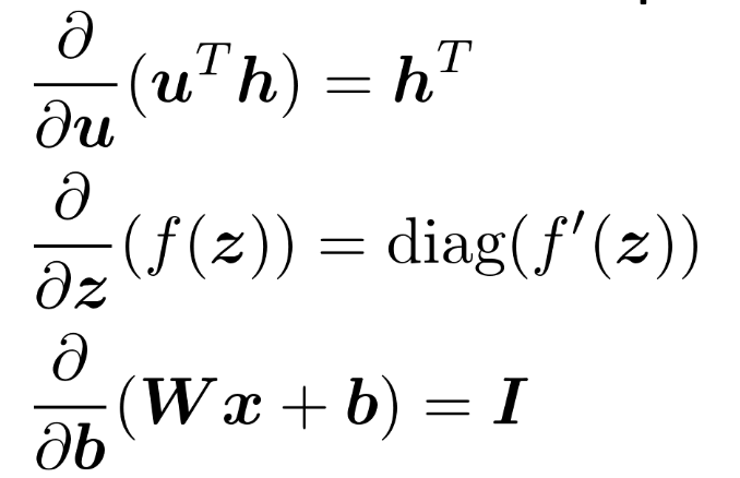
Why is the middle one?
Because the activations \(f\) are applied elementwise, only the diagonal are values and the off-diagonals are all \(0\) (because \(\pdv{h(x_1)}{x_2} = 0\)).
Shape Convention
We will always by output shape as the same shape of the parameters.
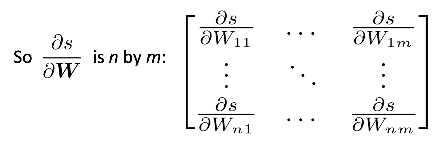
- shape convention: derivatives of matricies are the shape
- Jacobian form: derivatives w.r.t. matricies are row vectors
we use the first one
Actual Backprop
- create a topological sort of your computation graph
- calculate each variable in that order
- calculate backwards pass in reverse order
Check Gradient
\begin{equation} f’(x) \approx \frac{f(x+h) - f(x-h)}{2h} \end{equation}