perplexity
see perplexity
Vanishing Gradients
Consider how an RNN works: as your sequence gets longer, the earlier layers gets very little gradients because you have to multiply the gradient of each layer by the other.
Alternatively, if the gradient is very large, the parameter updates can blow up exponentially as well if your weights are too large (its either exponentially small or exponentially huge).
Why is this a problem?
To some extent, you can consider that we should tune the nearby weights a lot more than stuff way earlier than the sequence. Ham-fisting, we roughly have 7 tokens worth of effective conditioning.
However, this is EXPONENTIAL which is very bad, so we need to encode the gradient information into the nearby layers.
Also English has long-distance dependencies.
Solving Exploding Gradients
You can’t fix vanishing gradients, but fixing exploding gradient simply involves gradient clipping:
# rescale gradients to be at most `threshold` big
if gradients.norm() > threshold:
    gradients = gradients/(gradients.norm()) * threshold
Solving Vanishing Gradients
- LSTMs (additive accumulation)
- residual connections (skipping connections, see ResNet)
LSTM
This is actually proposed as a solution to RNN Vanishing Gradients:
\begin{equation} \begin{cases} f^{(t)} = \sigma \qty(W_{f}h^{(t-1)} + U_{f} x^{(t)} + b_{f}) \\ i^{(t)} = \sigma \qty(W_{i} h^{(t-1)} + U_{i} x^{(t)} + b_{i}) \\ o^{(t)} = \sigma \qty(W_{o} h^{(t-1)} + U_{o} x^{(t)} + b_{o}) \end{cases} \end{equation}
so for every single timestamps, we calculate three separate vector elements (one dimention per cell element) which controls how much you $f$orget, $i$nput to the memory cell, $o$utput to the current timestamp’s hidden layer.
From there, at each we first calculate a new cell at the current timestamp:
\begin{equation} \tilde{c}^{(t)} = \text{tanh} \qty(W_{c} h^{(t-1)} + U_{c} x^{(t)} + b_{c}) \end{equation}
and we actually put it into the cell by multiplying our gating values:
\begin{equation} c^{(t)} = f^{(t)} \odot c^{(t-1)} + i^{(t)} \odot \tilde{c}^{(t)} \end{equation}
and finally, we take a proportion:
\begin{equation} h^{(t)} = o^{(t)} \odot \text{tanh}\qty( c^{(t)}) \end{equation}
KEY SECRET: notice how the value of \(c^{(t)}\) is a PLUS SIGN between previous memory and current memory. At each point, our gradients are now ADDITIVE instead of multiplicative. LSTM architecture, therefore, allows you to preserve information across many timestamps.
Sentence Level LSTM Representation
LSTMs output its hidden state at every point. Therefore, its usually the best to take element-wise mean/max and use that as the sentence encoding to capture information about the entire sequence.
Bi-LSTM
To enable the understanding of both the information carried from both sides of the document, we can run a Bi-LSTM: whereby, the forward RNN run normally, the backward RNN reads backwards, and at every timestamp both of their directions’ embeddings are contacted.
Machine Translation
Statistical Machine Translation
Old-school translations used Bayes rule:
we want the best target sentence \(y\) given \(x\) input sentence, meaning:
\begin{equation} \arg\max_{y} P(y|x) \end{equation}
Using Bayes’ rule, we break it down into two parts:
\begin{equation} \arg\max_{y} P(x|y) P(y) \end{equation}
where the left side is a simple mapping between source phrases given target phrases, and the right is a language model to score how likely that ordering of phrases could be.
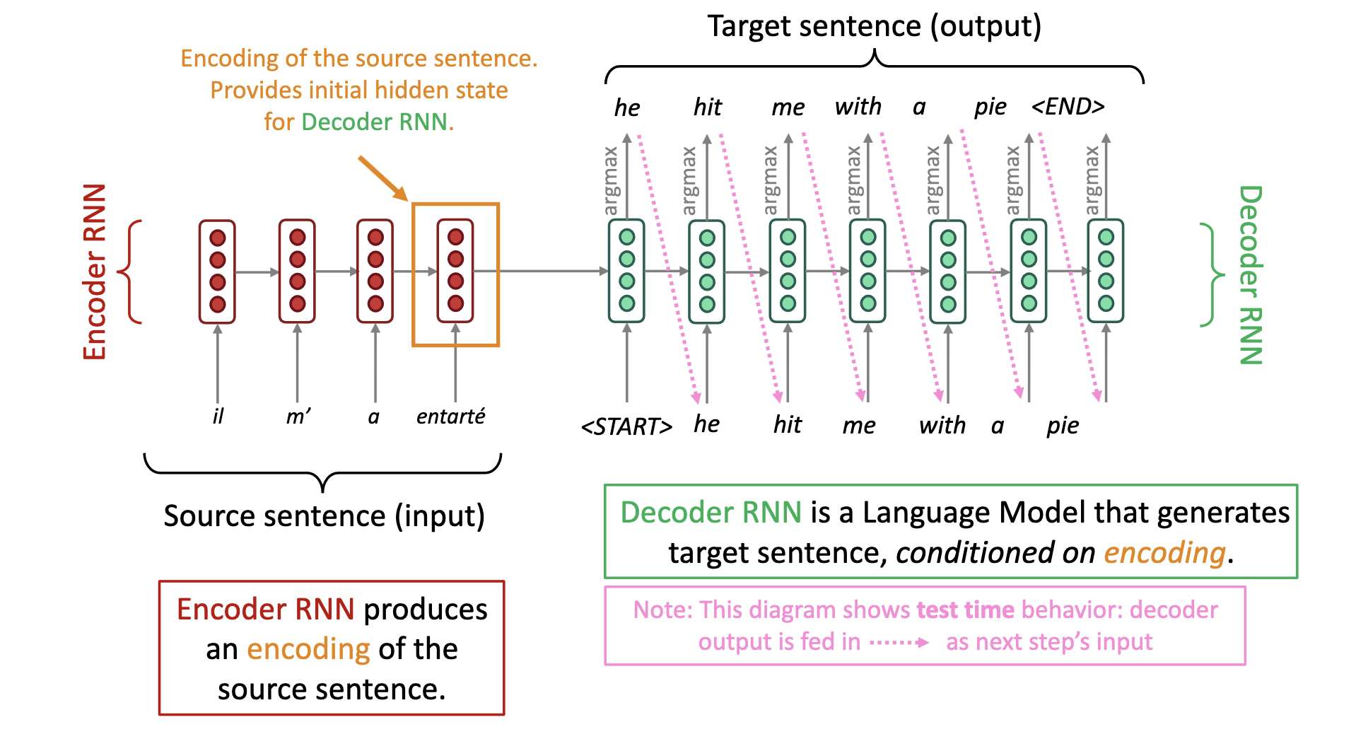
Neural Machine Translation
The above is bad. You can’t just reorder translated phrases and call that’s a good translation. So instead, we encoder-decoder: