More Bracketing Methods
Quadratic search
if your function is unimodal…
- Pick three points that gets “high, low, high”
- Fit a quadratic to it, evaluate its minima and add it to the point set
- Now, drop any of the four resulting point
Shubert-Piyavskill Method
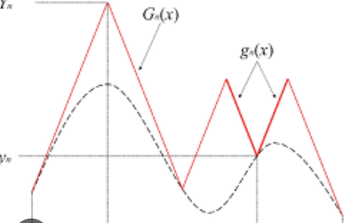
This is a Bracketing approach which grantees optimality WITHOUT unimodality by using the Lipschitz Constant. But, this only works in one dimension.
Consider a Lipschitz continuous function with Lipschitz Constant \(L\). We can get our two initial points \(a\) and \(b\). First, we arbitrarily pick a point in the middle to evaluate; this will give us a cone (see Lipschitz Condition) which bounds the function.
We will then evaluate the function + draw a new cone at each of our ed points \(a, b\). By piecing together the cones, we now obtain a sawtooth which lower bounds our function. We will continue this by choosing the lowest point on our lower bound, reevaluating, raising it to the new sawtooth.
For instance, in maximization, we can end up with sawtooths like:
Bisection Method
like Newton’s Method, this is a ROOT FINDING METHOD which we are coopting to find the minima by solving for FONC within an interval.
bisect \(f’(x)\) by sampling points in the middle of the “valid interval” until you find the point which gives \(f’(x) = 0\).
You do this by sampling points on each edge ensuring that there is a sign switch between each edge (i.e. there is a root between the edge points), and then sampling the middle of the interval. You know that there is a sign switch somewhere by the intermediate value theorem.
Local Descent
Descent Direction Iteration
Descent Direction Iteration is a class of method that uses a “local model” to improve the design point until we converge.
- check whether our current \(\bold{x}\) meets our termination conditions; if not…
- calculate some descent direction \(\bold{d}\) to update our \(\bold{x}\); sometimes, people say it has to be normalized
- decide some step size \(\alpha\)
- have fun: \(\bold{x} \leftarrow \bold{x} + \alpha \bold{d}\)
Line Search
We can choose the step size \(\alpha\) to perform using line search; i.e., figure out our \(\bold{d}\) somehow, and then use any of the Bracketing methods (or grid it up) to solve:
\begin{equation} \min_{\alpha} f(\bold{x} + \alpha \bold{d}) \end{equation}
Decaying \(\alpha\)
We can also give up solving for the greatest \(\alpha\), fix a learning rate, and then decay it using \(\alpha \gamma^{n}\) where \(n\) is the number of iterations and \(\gamma\) is the decay rate.
Approximate Line Search
Instead of continuously evaluating the function \(f\), we use a first order approximation on our directional derivative (plus some acceptability factor \(\beta \in [0,1]\), usually \(\beta=1 \times 10^{-4}\)).
We will then choose the largest \(\alpha\) that satisfies
Sufficient Decrease Condition
\begin{equation} f(x_{t+1}) \leq f(x_{t}) + \beta \alpha \nabla_{d} f(x_{t}) \end{equation}
Curvature Condition
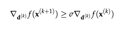
which bounds the “shallowness” of the directional derivatives.
Trust Region Methods
We often want to bound our change in \(x\) by some region \(\delta\) in our steps; so, we really want to…
\begin{align} \min_{x’}\ &f(x’) \\ s.t.\ & \mid x-x’ \mid \leq \delta \end{align}
To figure \(\delta\), we shrink our region of trust based on the quality of our function estimate (if we used a first-order local model to figure our descent direction, we will use our first order estimate for \(\hat{f}\)):
\begin{align} \eta = \frac{f(x)-f(x’)}{f(x)-\hat{f}(x’)} \end{align}
if \(\eta < \eta_{1}\), we would scale down \(\delta\) by some amount as evidently our actual improvement is smaller than expected and reject our new point; if \(\eta > \eta_{2}\), we will accept our new point and scale up \(\delta\) by some amount as our improvement is better than expected. Otherwise, we will accept the new point an do not nothing to the trust region.
Termination Conditions
Maximum Iterations
\begin{equation} k > k_{\max } \end{equation}
termination condition for those on a deadline
Absolute Improvement
\begin{equation} |f(x_{t}) - f(x_{t+1})| < \epsilon \end{equation}
Relative Improvement
\begin{equation} f(x_{t}) - f(x_{t+1}) < \epsilon | f(x)| \end{equation}
Some range of acceptability.
Gradient
\begin{equation} |\nabla f(x_{t})| < \epsilon \end{equation}
First-Order Methods
gradient descent
see gradient descent
\begin{equation} \bold{d} = \nabla f(x) \end{equation}
Conjugate Gradient
Motivation: steepest-design, but choose search directions that is orthogonal to \(A\)! Suppose \(A\) is symmetric, positive-definite. Choosing orthogonal search directions helps us preclude searching in overlapping directions (and wasting time).
Essentially, we choose: \(\langle s^{^{(q)}}, s^{^{(\hat{q})}} \rangle_{A}\) with \(A\) weighted Matrix-scaled inner product. (“Orthogonality carries regardless of weighting”).
We optimize the function as if its a gradratic function:
\begin{equation} \min_{x} f(x) = \frac{1}{2} \bold{x}^{\top} \bold{A}\bold{x} + \bold{b}^{\top} \bold{x} + c \end{equation}
where \(A\) is a positive, definite matrix. Under this assumption, we consider that this function would behave like a bowl.
We can then formulate:
\begin{equation} \bold{d}_{t+1} = -\nabla_{t+1} f + \beta \bold{d}_{t} \end{equation}
where \(\bold{d}_{t+1}\) is the step direction we are going to use at t+2!! So we are essentially averaging the direction from two steps before.
We usually set \(\beta\) to be the Fletcher-Reeves or Polak-Ribere approaches.
All descent direction are Mutually Conjugate.
Mutually Conjugate
if \(x_{i} \neq x_{j}\) are Mutually Conjugate, we have:
\begin{equation} x_{i} A x_{j} = 0 \end{equation}
Error-Analysis for Conjugate Gradient
“Steepest Descent/gradient descent, but choose step directions to be \(A\) orthogonal instead”
Initial error \(e^{(1)} = \sum_{\hat{q} = 1}^{n} \beta^{\hat{(q)}} s^{\hat{(q)}}\) (\(\beta\) is the coefficients that we don’t know, which are the things we want to solve for which gives us the error.)
\begin{equation} e^{(q)} = e^{(1)} + \sum_{\hat{q} = 1}^{q-1} \alpha^{(\hat{q})} s^{(\hat{q})} \end{equation}
this implies that:
\begin{equation} \langle s^{(q)}, e^{(q)} \rangle_{A} = \langle s^{(q)}, e^{(1)} \rangle_{A} \end{equation}
this gives:
\begin{equation} \alpha^{(q)} = \frac{s^{(q)}r^{(q)}}{s^{(q)} A s^{(q)}} = - \frac{\langle s^{(q)}, e^{(q)} \rangle}{\langle s^{(q)},s^{(q)} \rangle_{A}} = -\beta^{(q)} \end{equation}
meaning: if all \(s\) are \(A\) orthogonal, the \(\alpha\) choices will result in convergence in \(n\) steps. Note that if residuals \(\tilde{q} < q\), then \(s^{\tilde{q}} \cdot r^{q} = -\langle s^{\tilde{q}}, e^{q} \rangle_{A} = 0\). Meaning, residuals are orthogonal to all previous search directions.
Momentum
We descent by calculating a “position” and a “velocity”
\begin{equation} v_{t+1} = \beta v_{t} - \alpha \nabla_{x_{t}} f \end{equation}
\begin{equation} x_{t+1} = x_{t} + v_{t+1} \end{equation}
if \(\beta\), the momentum is set to \(0\), we just get normal gradient descent. If there is a positive \(\beta\), your update vector will take on some of the previous update direction values.