constraint
recall constraint; our general constraints means that we can select \(f\) within a feasible set \(x \in \mathcal{X}\).
active constraint
an “active constraint” is a constraint which, upon application, changes the solution to be different than the non-constrainted solution. This is always true at the equality constraint, and not necessarily with inequality constraints.
types of constraints
We can write all types of optimization problems into two types of constraints; we will use these conventions EXACTLY:
equality
situations where:
\begin{equation} h(\bold{x}) = 0 \end{equation}
“some transformation on \(x\) must result in \(0\)”
we can transform all constraints to this type trivially:
\begin{equation} h(x) = \bold{1}\qty(x \not\in \mathcal{X}) = 0 \end{equation}
inequality
situations where:
\begin{equation} g(\bold{x}) \leq 0 \end{equation}
“some transformation on \(x\) must be non-positive”
region-based constraints
if we want \(x \in [a,b]\), we can transform this into an unconstrained optimization problem by substituting the rescaled version into the input:
\begin{equation} x\qty(\hat{x}) = \frac{b+a}{2} + \frac{b-a}{2} \qty( \frac{2 \hat{x}}{1+ \hat{x}^{2}}) \end{equation}
you can choose any transformation that keeps you into the you can choose any transformation that keeps you into the you can choose any transformation that keeps you into the you can choose any transformation that keeps you into the feasible set (say, sigmoid).
Lagrange multiplier
“the gradient of the objective function has to be perpendicular to the gradient of the constraints”
For Equality constraints
Assume we only have an equality constraint:
\begin{align} \min_{x}&\ f(x)\\ s.t.&\ h(x) = 0 \end{align}
We are going to create a Lagrangian of this system:
\begin{equation} \mathcal{L}(x, \lambda) = f(x) - \lambda h(x) \end{equation}
Setting the gradient of this to \(0\):
\begin{equation} \nabla \mathcal{L} = 0 = f’(x) - \lambda h’(x) \end{equation}
meaning:
\begin{equation} f’(x) = \lambda h’(x) \end{equation}
We can now also recall that \(h(x) = 0\). We now have a system:
\begin{equation} \begin{cases} f’(x) = \lambda h’(x) \\ h(x) = 0 \end{cases} \end{equation}
We can go now to solve for \(x, \lambda\).
For Inequality constraints
\begin{align} \min_{x}&\ f(x)\\ s.t.&\ g(x) \leq 0 \end{align}
We have (we switched the signs, but it doesn’t matter):
\begin{equation} \mathcal{L}(x, \mu) = f(x) + \mu g(x) \end{equation}
Combined
\begin{equation} \mathcal{L}(x, \mu, \lambda) = f(x) + \mu g(x) + \lambda h(x) \end{equation}
Infinite step function
We now formulate this such that boundaries outside of the constraints is infinitely large; recall that our constraint have \(g(x) \leq 0\). Meaning:
\begin{equation} f_{\infty} = \max_{\mu \geq 0} \mathcal{L}(x, \mu) = \max_{\mu \geq 0} \qty(f(x) + \mu g(x)) \end{equation}
this uses the fact that, at feasible \(g\) (i.e. non-positive \(g\)), the most optimal choice of \(\mu\) is \(0\), whereas at non-feasible \(g\), the optimal is \(\mu \to \infty\).
Meaning, our problem becomes:
primal problem
\begin{equation} \min_{x} \max_{\mu \geq 0, \lambda} \mathcal{L}(x,\mu, \lambda) \end{equation}
KKT Conditions
feasibility
364a notation
primal feasible: \(f_{i}\qty(x) \leq 0, h_{i} = 0\)
222 notation
\begin{equation} \begin{cases} g(x^{*}) \leq 0 \\ h(x^{*}) = 0 \end{cases} \end{equation}
dual feasibility
364a notation
\begin{equation} \lambda \geq 0 \end{equation}
222 notation
\begin{equation} \mu \geq 0 \end{equation}
complementary slackness
364a notation
Complementary Slackness: \(\lambda_{i} f_{i}\qty(x) = 0\) for all \(i\)
222 notation
\begin{equation} u \cdot g = 0 \end{equation}
stationarity
364a notation
gradient of the Lagrangian wrt \(x\) vanishes. That is, \(\nabla_{x} L\qty(x, \lambda, v) = 0\).
i.e. we got the infinitum by \(x\)
222 notation
objective function is tangent to each constraint
\begin{equation} \nabla f(x) + \mu \nabla g(x) + \lambda \nabla h(x) = 0 \end{equation}
dual form of the primal problem
we can incorporate our active constraint term to write:
\begin{equation} \mathcal{L}(x, \mu, \lambda) = f(x) + \mu \cdot g(x) + \lambda \cdot h(x) \end{equation}
by the same principle above, we can write:
\begin{equation} \min_{x} \max_{\mu \geq 0, \lambda} \mathcal{L}(x,\mu, \lambda) \end{equation}
we now write the DUAL of this function:
\begin{equation} \mathcal{D} = \max_{\mu \geq 0, \lambda} \min_{x} \mathcal{L}(x,\mu, \lambda) \end{equation}
by the min-max duality theorem, we now that solutions to this will bound the actual primal problem. The difference between \(\mathcal{D}\) and the primal problem is called the duality gap.
min-max duality theorem
\begin{align} \max_{a} \min_{b} f(a,b) \leq \min_{b} \max_{a} f(a,b) \end{align}
for any function \(f(a,b)\). Therefore, the solution to the dual problem is a lower bound to the primal solution.
Penalty Methods
We use these methods if we are outside of the KKT Conditions, which will bring us into those conditinos. We can use the Lagrange multiplier conditions to reshape a constrained problem into a unconstrained one to satisfy the KKT Conditions.
count penalty, quadratic penalty, and mixed penalty.
We just write it:
\begin{equation} \min_{x} f(x) + \rho p \end{equation}
where \(p\) comes from
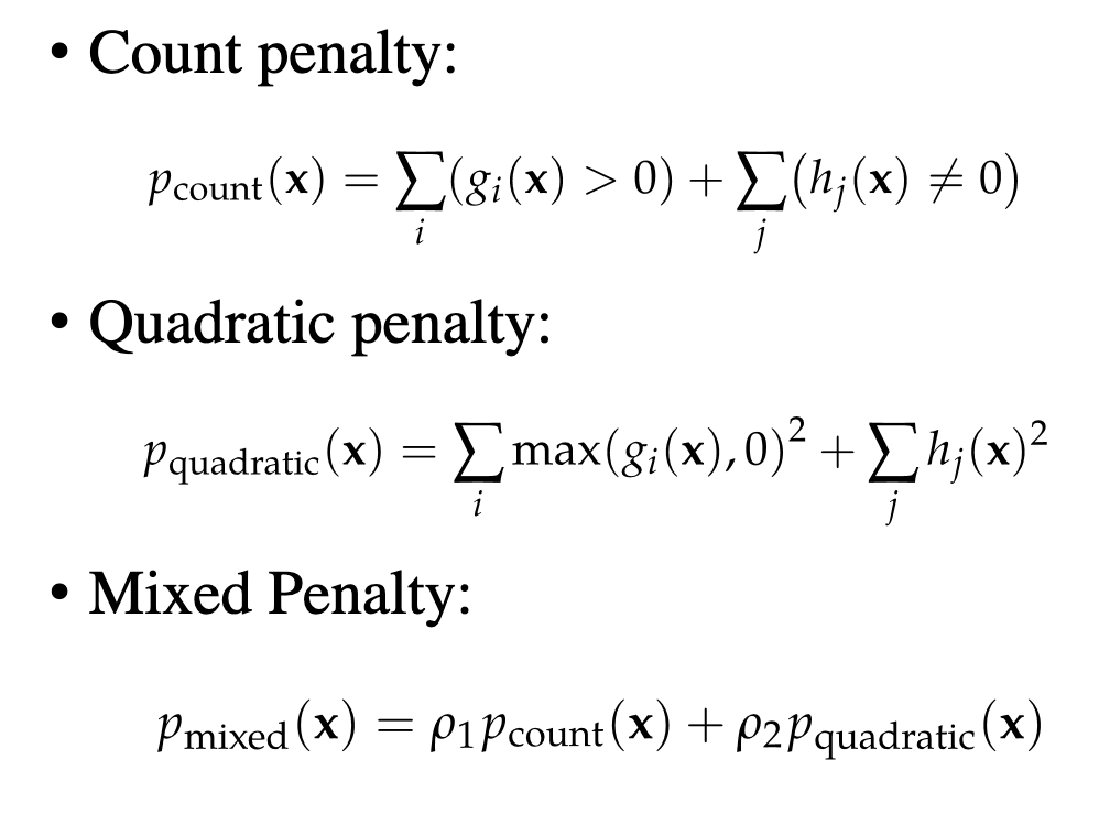
over time for solving the function, we slowly rachet up \(\rho\) until \(\rho \to \infty\) until we reach it as a hard limit.