digital encoding
We allocating different systems in the same environment different frequency bands; by doing this, we are able to communicate pack information more effectively to prevent interference.
“how do we take a sequence of bits 10100…. and map it to a continuous-time signal \(X(t)\) such that the spectrum of this system is limited to \([0, B]\)”?
sinc digital encoding
IDEA: recall sinc sampling theorem, which (even if under sampled), will recover the source points exactly. As such, we can write:
\begin{equation} X(t) = \sum_{m=1}^{\infty} X[m] \text{sinc} \qty( \frac{t-mT}{T}) \end{equation}
for your choice of period \(T > 0\). where, \(X[m] = V \cdot b_{m}\) where \(b_{m}\) is the binary (Huffman Coding) encoding of your data.
By the sinc sampling theorem, we know that the spectrum of the recovered signal would be at most \(\frac{1}{2}T\), where \(T\) is the rate of our data. This makes the rate of our communication to be \(\frac{1}{T}\) bits per second. If we have a maximum bandwidth alliance of \(B\), then, this means our rate of communication is \(2B\) (higher the bandwidth, higher the speed).
The sinc function gets the smallest possible bandwidth for each sampling frequency.
passband digital encoding
digital encoding schemes we described gives Baseband Signals. But, we are usually allocated a Passband Signal range (i.e. we can’t use lower bands).
so, we would like to communicate a \(2B\) Bandwidth whereby:
\begin{equation} \mathcal{F}(X(t)) \in [f_{c} -B, f_{c} + B] \end{equation}
where the Bandwidth is still \(2B\).
Typically, \(f_{c} \gg b\).
We also want this because as frequency decreases, antennae size (i.e. wavelength) needs to increase. Therefore, we want to typically use a small bandwidth within a high frequency range.
Consider now the fact that:
\begin{equation} 2 \sin B\cos f_{c} = \sin (f_{c}+B) + \sin (f_{c} -B) \end{equation}
you will note that this gives us exactly two signals, with frequencies \(f_{c}\pm B\), and a bandwidth of \(2B\).
This means that, once you get your baseband signal of frequency \(B\), we can project it into something centered around \(f_{c}\) with bandwidth \(2B\) by mutliplying by \(\cos \qty(2 \pi f_{c})\).
decoding
Because we are no longer on-off keying, decoding becomes more of a challenge. If your frequency is too quick, you need to figure out a way if a \(0\) you sampled is really no data or whenever the way you happened to get at the \(0\).
Instead of doing this, recall that a signal would look like
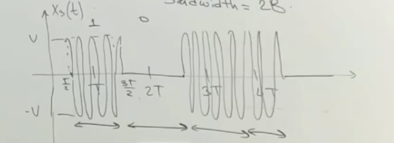
So, assuming you are synchronized with the transmitted squak, you’d expect that the integral at every period would be high, then low, etc. Recall:
\begin{equation} \varepsilon_{m} = \int_{mT - \frac{T}{2}}^{mT + \frac{T}{2}} y^{2}(t) \dd{t} \end{equation}
is the energy corresponding to the \(m\) th timeslot. Consider a timeslot when the signval is on
\begin{equation} \int_{0}^{T} V^{2} \cos^{2} \qty(2 \pi f_{c} t) \dd{t} \approx \frac{V^{2}T}{2} = \varepsilon_{m} \end{equation}
we expect that this integral/computation gives us near-zero when \(V = 0\). So we will set some thresholds for \(\varepsilon\) at each sample.
sync
have a preamble to sync things up.