CAPM, a Review
Note that we will be using the Sharpe-Linter version of CAPM:
\begin{equation} E[R_{i}-R_{f}] = \beta_{im} E[(R_{m}-R_{f})] \end{equation}
\begin{equation} \beta_{im} := \frac{Cov[(R_{i}-R_{f}),(R_{m}-R_{f})]}{Var[R_{m}-R_{f}]} \end{equation}
Recall that we declare \(R_{f}\) (the risk-free rate) to be non-stochastic.
Let us begin. We will create a generic function to analyze some given stock.
Data Import
We will first import our utilities
import pandas as pd
import numpy as np
Let’s load the data from our market (NYSE) as well as our 10 year t-bill data.
t_bill = pd.read_csv("./linearity_test_data/10yrTBill.csv")
nyse = pd.read_csv("./linearity_test_data/NYSEComposite.csv")

nyse.head()
                  Date     Close
0   11/7/2013 16:00:00   9924.37
1   11/8/2013 16:00:00  10032.14
2  11/11/2013 16:00:00  10042.95
3  11/12/2013 16:00:00  10009.84
4  11/13/2013 16:00:00  10079.89
Excellent. Let’s load in the data for that stock.
def load_stock(stock):
    return pd.read_csv(f"./linearity_test_data/{stock}.csv")

load_stock("LMT").head()
                  Date   Close
0   11/7/2013 16:00:00  136.20
1   11/8/2013 16:00:00  138.11
2  11/11/2013 16:00:00  137.15
3  11/12/2013 16:00:00  137.23
4  11/13/2013 16:00:00  137.26
Raw Data
And now, let’s load all three stocks, then concatenate them all into a big-ol DataFrame.
# load data
df = { "Date": nyse.Date,
       "NYSE": nyse.Close,
       "TBill": t_bill.Close,
       "LMT": load_stock("LMT").Close,
       "TWTR": load_stock("TWTR").Close,
       "MCD": load_stock("MCD").Close }

# convert to dataframe
df = pd.DataFrame(df)
# drop empty
df.dropna(inplace=True)

df
                     Date      NYSE  TBill     LMT   TWTR     MCD
0      11/7/2013 16:00:00   9924.37  26.13  136.20  44.90   97.20
1      11/8/2013 16:00:00  10032.14  27.46  138.11  41.65   97.01
2     11/11/2013 16:00:00  10042.95  27.51  137.15  42.90   97.09
3     11/12/2013 16:00:00  10009.84  27.68  137.23  41.90   97.66
4     11/13/2013 16:00:00  10079.89  27.25  137.26  42.60   98.11
...                   ...       ...    ...     ...    ...     ...
2154  10/24/2022 16:00:00  14226.11  30.44  440.11  39.60  252.21
2155  10/25/2022 16:00:00  14440.69  31.56  439.30  39.30  249.28
2156  10/26/2022 16:00:00  14531.69  33.66  441.11  39.91  250.38
2157  10/27/2022 16:00:00  14569.90  34.83  442.69  40.16  248.36
2158  10/28/2022 16:00:00  14795.63  33.95  443.41  39.56  248.07

[2159 rows x 6 columns]
Log Returns
Excellent. Now, let’s convert all of these values into daily log-returns (we don’t really care about the actual pricing.)
log_returns = df[["NYSE", "TBill", "LMT", "TWTR", "MCD"]].apply(np.log, inplace=True)
df.loc[:, ["NYSE", "TBill", "LMT", "TWTR", "MCD"]] = log_returns
df
                     Date      NYSE     TBill       LMT      TWTR       MCD
0      11/7/2013 16:00:00  9.202749  3.263084  4.914124  3.804438  4.576771
1      11/8/2013 16:00:00  9.213549  3.312730  4.928050  3.729301  4.574814
2     11/11/2013 16:00:00  9.214626  3.314550  4.921075  3.758872  4.575638
3     11/12/2013 16:00:00  9.211324  3.320710  4.921658  3.735286  4.581492
4     11/13/2013 16:00:00  9.218298  3.305054  4.921877  3.751854  4.586089
...                   ...       ...       ...       ...       ...       ...
2154  10/24/2022 16:00:00  9.562834  3.415758  6.087025  3.678829  5.530262
2155  10/25/2022 16:00:00  9.577805  3.451890  6.085183  3.671225  5.518577
2156  10/26/2022 16:00:00  9.584087  3.516310  6.089294  3.686627  5.522980
2157  10/27/2022 16:00:00  9.586713  3.550479  6.092870  3.692871  5.514879
2158  10/28/2022 16:00:00  9.602087  3.524889  6.094495  3.677819  5.513711

[2159 rows x 6 columns]
And now, the log returns! We will shift this data by one column and subtract.
returns = df.drop(columns=["Date"]) - df.drop(columns=["Date"]).shift(1)
returns.dropna(inplace=True)
returns
          NYSE     TBill       LMT      TWTR       MCD
1     0.010801  0.049646  0.013926 -0.075136 -0.001957
2     0.001077  0.001819 -0.006975  0.029570  0.000824
3    -0.003302  0.006161  0.000583 -0.023586  0.005854
4     0.006974 -0.015657  0.000219  0.016568  0.004597
5     0.005010 -0.008476  0.007476  0.047896 -0.005622
...        ...       ...       ...       ...       ...
2154  0.005785  0.004940 -0.023467 -0.014291  0.001349
2155  0.014971  0.036133 -0.001842 -0.007605 -0.011685
2156  0.006282  0.064420  0.004112  0.015402  0.004403
2157  0.002626  0.034169  0.003575  0.006245 -0.008100
2158  0.015374 -0.025590  0.001625 -0.015053 -0.001168

[2158 rows x 5 columns]
Risk-Free Excess
Recall that we want to be working with the excess-to-risk-free rates \(R_{T}-R_{f}\), where \(R_{T}\) is some security. So, we will go through and subtract everything by the risk-free rate (and drop the RFR itself):
risk_free_excess = returns.drop(columns="TBill").apply(lambda x: x-returns.TBill)
risk_free_excess
          NYSE       LMT      TWTR       MCD
1    -0.038846 -0.035720 -0.124783 -0.051603
2    -0.000742 -0.008794  0.027751 -0.000995
3    -0.009463 -0.005577 -0.029747 -0.000307
4     0.022630  0.015875  0.032225  0.020254
5     0.013486  0.015952  0.056372  0.002854
...        ...       ...       ...       ...
2154  0.000845 -0.028406 -0.019231 -0.003591
2155 -0.021162 -0.037975 -0.043738 -0.047818
2156 -0.058138 -0.060308 -0.049017 -0.060017
2157 -0.031543 -0.030593 -0.027924 -0.042269
2158  0.040964  0.027215  0.010537  0.024422

[2158 rows x 4 columns]
Actual Regression
It is now time to perform the actual linear regression! We will use statsmodels’ Ordinary Least Squares API to make our work easier, but we will go through a full regression in the end.
import statsmodels.api as sm
CAPM Regression: Lockheed Martin
Let’s work with Lockheed Martin first for regression, fitting an ordinary least squares. Remember that the OLS functions reads the endogenous variable first (for us, the return of the asset.)
# add a column of ones to our input market excess returns
nyse_with_bias = sm.add_constant(risk_free_excess.NYSE)

# perform linreg
lmt_model = sm.OLS(risk_free_excess.LMT, nyse_with_bias).fit()

lmt_model.summary()
                            OLS Regression Results
==============================================================================
Dep. Variable:                    LMT   R-squared:                       0.859
Model:                            OLS   Adj. R-squared:                  0.859
Method:                 Least Squares   F-statistic:                 1.312e+04
No. Observations:                2158   AIC:                        -1.263e+04
Df Residuals:                    2156   BIC:                        -1.262e+04
Df Model:                           1   Prob (F-statistic):               0.00
Covariance Type:            nonrobust   Log-Likelihood:                 6318.9
==============================================================================
                 coef    std err          t      P>|t|      [0.025      0.975]
------------------------------------------------------------------------------
const          0.0004      0.000      1.311      0.190      -0.000       0.001
NYSE           0.9449      0.008    114.552      0.000       0.929       0.961
==============================================================================
Based on the constants row, we can see that—within \(95\%\) confidence—the intercept is generally \(0\) and CAPM applies. However, we do see a slight positive compared to the market. Furthermore, we can see that the regression has a beta value of \(0.9449\) — according the CAPM model, it being slightly undervarying that the market.
CAPM Regression: MacDonald’s
# perform linreg
mcd_model = sm.OLS(risk_free_excess.MCD, nyse_with_bias).fit()

mcd_model.summary()
                            OLS Regression Results
==============================================================================
Dep. Variable:                    MCD   R-squared:                       0.887
Model:                            OLS   Adj. R-squared:                  0.887
Method:                 Least Squares   F-statistic:                 1.697e+04
No. Observations:                2158   AIC:                        -1.310e+04
Df Residuals:                    2156   BIC:                        -1.309e+04
Df Model:                           1   Prob (F-statistic):               0.00
Covariance Type:            nonrobust   Log-Likelihood:                 6551.1
==============================================================================
                 coef    std err          t      P>|t|      [0.025      0.975]
------------------------------------------------------------------------------
const          0.0003      0.000      1.004      0.315      -0.000       0.001
NYSE           0.9651      0.007    130.287      0.000       0.951       0.980
==============================================================================
Same thing as before, we are within \(95\%\) confidence having a intercept of \(0\) (with a slight positive edge), and it looks like MacDonald’s vary a little bit more than Lockheed Martin. The food industry is probably a tougher business than that in defense.
CAPM Regression: Twitter
Lastly, to analyze the recently delisted Twitter!
# perform linreg
twtr_model = sm.OLS(risk_free_excess.TWTR, nyse_with_bias).fit()

twtr_model.summary()
                            OLS Regression Results
==============================================================================
Dep. Variable:                   TWTR   R-squared:                       0.522
Model:                            OLS   Adj. R-squared:                  0.522
Method:                 Least Squares   F-statistic:                     2357.
No. Observations:                2158   AIC:                            -8610.
Df Residuals:                    2156   BIC:                            -8599.
Df Model:                           1   Prob (F-statistic):               0.00
Covariance Type:            nonrobust   Log-Likelihood:                 4307.1
==============================================================================
                 coef    std err          t      P>|t|      [0.025      0.975]
------------------------------------------------------------------------------
const         -0.0002      0.001     -0.346      0.730      -0.002       0.001
NYSE           1.0173      0.021     48.549      0.000       0.976       1.058
==============================================================================
Evidently, Twitter is much more variable. It looks like it has a nontrivial bias (the intercept being -0.001 being within the \(95\%\) confidence band — that the security is possibly significantly underperforming the CAPM expectation in the market.) Furthermore, we have a positive beta value: that the asset is more variable than the market.
Manual Checking
We can also use the betas formula to manually calculate what we expect for the beta values (i.e. as if they were one IID random variable.)
risk_free_cov = risk_free_excess.cov()
risk_free_cov
          NYSE       LMT      TWTR       MCD
NYSE  0.001143  0.001080  0.001163  0.001103
LMT   0.001080  0.001188  0.001116  0.001083
TWTR  0.001163  0.001116  0.002264  0.001155
MCD   0.001103  0.001083  0.001155  0.001200
Finally, to construct the beta values. Recall that:
\begin{equation} \beta_{im} := \frac{Cov[(R_{i}-R_{f}),(R_{m}-R_{f})]}{Var[R_{m}-R_{f}]} \end{equation}
and that:
\begin{equation} Var[X] = Cov[X,X], \forall X \end{equation}
# get the market variance (covariance with itself)
market_variation = risk_free_cov.NYSE.NYSE

# calculate betas
betas = {"LMT": (risk_free_cov.LMT.NYSE/market_variation),
         "TWTR": (risk_free_cov.TWTR.NYSE/market_variation),
         "MCD": (risk_free_cov.MCD.NYSE/market_variation)}

# and make dataframe
betas = pd.Series(betas)
betas
LMT     0.944899
TWTR    1.017294
MCD     0.965081
dtype: float64
Apparently, all of our assets swing less than the overall NYSE market! Especially Lockheed—it is only \(94.4\%\) of the market variation. Furthermore, it is interesting to see that Twitter swings much more dramatically compared to the market.
Equal-Part Fund
We will now create two funds with the three securities, one with equal parts and one which attempts to maximizes the bias (max returns) while minimizing the beta variance value compared to the market.
First, let’s create a baseline fund in equal parts. Here it is:
fund_1_returns = returns.LMT + returns.TWTR + returns.MCD
fund_1_returns
1      -0.063167
2       0.023420
3      -0.017149
4       0.021384
5       0.049750
          ...
2154   -0.036409
2155   -0.021132
2156    0.023917
2157    0.001720
2158   -0.014596
Length: 2158, dtype: float64
We will calculate the excess returns of this fund:
fund_1_excess = fund_1_returns-returns.TBill
fund_1_excess
1      -0.112813
2       0.021600
3      -0.023310
4       0.037041
5       0.058226
          ...
2154   -0.041349
2155   -0.057265
2156   -0.040503
2157   -0.032449
2158    0.010994
Length: 2158, dtype: float64
Performance of the Equal-Part Fund
# perform linreg
fund_1_model = sm.OLS(fund_1_excess, nyse_with_bias).fit()

fund_1_model.summary()
                            OLS Regression Results
==============================================================================
Dep. Variable:                      y   R-squared:                       0.473
Model:                            OLS   Adj. R-squared:                  0.473
Method:                 Least Squares   F-statistic:                     1935.
No. Observations:                2158   AIC:                            -7735.
Df Residuals:                    2156   BIC:                            -7724.
Df Model:                           1   Prob (F-statistic):          3.01e-302
Covariance Type:            nonrobust   Log-Likelihood:                 3869.5
==============================================================================
                 coef    std err          t      P>|t|      [0.025      0.975]
------------------------------------------------------------------------------
const          0.0007      0.001      0.841      0.401      -0.001       0.002
NYSE           1.1290      0.026     43.993      0.000       1.079       1.179
==============================================================================
Surprisingly, we have now created a significantly riskier investment that, though riskier, generates a much higher probability of reward (\(+0.001\) is now within the \(99\%\) band!)
A More Optimized Fund
To me, this is the payoff of this assignment. We will now use CAPM to create the “best” fund combination—given some variance, the funds which match CAPM. To do this, let’s create a generic linear combination of the assets.
import sympy as sym
x = sym.Symbol('x')
y = sym.Symbol('y')
z = sym.Symbol('z')

fund_2_returns = x*returns.LMT + y*returns.TWTR + z*returns.MCD
fund_2_returns
1       0.0139260753744255*x - 0.0751364261353569*y - ...
2       -0.00697525170622448*x + 0.0295704573211193*y ...
3       0.000583132897928884*x - 0.0235859990058791*y ...
4       0.000218587198947517*x + 0.016568426347233*y +...
5       0.00747599199607762*x + 0.0478955096700351*y -...
                              ...
2154    -0.0234665578621085*x - 0.0142913301107561*y +...
2155    -0.00184214468578059*x - 0.0076045993852194*y ...
2156    0.00411172646842317*x + 0.0154024001854269*y +...
2157    0.00357547337231878*x + 0.0062445563228315*y -...
2158    0.00162509910496933*x - 0.0150529686289622*y -...
Length: 2158, dtype: object
Excellent. We will also calculate the excess returns of this fund:
fund_2_excess = fund_2_returns-returns.TBill
Y = fund_2_excess.to_numpy()
Y
[0.0139260753744255*x - 0.0751364261353569*y - 0.00195664549320096*z - 0.0496463208073039
 -0.00697525170622448*x + 0.0295704573211193*y + 0.000824317408861575*z - 0.00181917459665826
 0.000583132897928884*x - 0.0235859990058791*y + 0.00585367525146019*z - 0.00616055581298536
 ...
 0.00411172646842317*x + 0.0154024001854269*y + 0.00440300114913317*z - 0.0644196927849867
 0.00357547337231878*x + 0.0062445563228315*y - 0.0081004573348249*z - 0.0341688956152497
 0.00162509910496933*x - 0.0150529686289622*y - 0.00116834209450634*z + 0.0255902303732043]
We cast this type to a numpy array because we are about to perform some matrix operations upon it.
Optimizing the Optimized Fund: Linreg
Now, let us perform the actual linear regression ourselves. Recall that the pseudoinverse linear regression estimator is:
\begin{equation} \beta = (X^{T}X)^{-1}X^{T}Y \end{equation}
We have already our \(Y\) as a vector (above), and our \(X\) is:
X = nyse_with_bias.to_numpy()
X
[[ 1.00000000e+00 -3.88457302e-02]
 [ 1.00000000e+00 -7.42217926e-04]
 [ 1.00000000e+00 -9.46284244e-03]
 ...
 [ 1.00000000e+00 -5.81378271e-02]
 [ 1.00000000e+00 -3.15429207e-02]
 [ 1.00000000e+00  4.09643405e-02]]
We now have our matrices, let’s perform the linear regression!
linear_model = np.linalg.inv((X.transpose()@X))@X.transpose()@Y
linear_model
[0.000544056413840724*x - 6.62061061591867e-5*y + 0.000429966553373172*z - 0.000178620725465344
 0.0457830563134785*x + 0.118178191274045*y + 0.0659651260604729*z + 0.899115719100281]
Excellent. So we now have two rows; the top row represents the “bias”—how much deviation there is from CAPM, and the bottom row represents the “rate”—the “beta” value which represents how much excess variance there is.
Optimizing the Optimized Fund: Picking Optimizing Parameters
We can will solve for a combination of solutions to give us specific values of returns vs risk. For instance, we can fix the variance to 1 (i.e. we can vary as much as the market.) We subtract one here for the solver, which expects the expressions equaling to \(0\).
risk_expr = linear_model[1] - 1
risk_expr
0.0457830563134785*x + 0.118178191274045*y + 0.0659651260604729*z - 0.100884280899719
Now, we will set a certain earning value, and solve for possible solutions. We will try to get the largest possible bias without needing to short something (i.e. cause a negative solution). By hand-fisting a value, it seems 0.001 is a good bet.
deviance_expr = linear_model[0] - 0.001
deviance_expr
0.000544056413840724*x - 6.62061061591867e-5*y + 0.000429966553373172*z - 0.00117862072546534
Optimizing the Optimized Fund: Optimize!
solution = sym.solvers.solve([deviance_expr, risk_expr], x,y,z)
solution
{x: 2.16803104555387 - 0.819584899551304*z, y: 0.0137520589394366 - 0.24067066980814*z}
We have one degree of freedom here: how much MacDonald’s we want! Let’s say we want none (which would, according to this, be an equally efficient solution.)
How Does Our Fund Do?
This would create the following plan:
# for our case
z_val = 0
# numerical solutions
s_x = solution[x].subs(z,z_val)
s_y = solution[y].subs(z,z_val)

# solution
fund_2_nobias_nomac = s_x*returns.LMT + s_y*returns.TWTR + z_val*returns.MCD
fund_2_nobias_nomac.mean()
0.001185050286566688
Recall that this is the performance of the balanced portfolio:
fund_1_returns.mean()
0.0009224705380695683
So, for market-level risk (\(\beta =1\), instead of the balanced portfolio’s \(\beta =1.1290\)), this is a pretty good deal!
Some Plots
Finally, let’s plot the prices of our various funds:
import matplotlib.pyplot as plt
import matplotlib.dates as mdates
import seaborn as sns
from datetime import datetime

sns.set()

fund_2_price = s_x*df.LMT + s_y*df.TWTR + z_val*df.MCD
fund_1_price = df.LMT + df.TWTR
fund_l_price = df.LMT
fund_t_price = df.TWTR

dates = df.Date.apply(lambda x:datetime.strptime(x, "%m/%d/%Y %H:%M:%S"))

sns.lineplot(x=dates, y=fund_2_price.apply(sym.Float).astype(float))
sns.lineplot(x=dates, y=fund_1_price.apply(sym.Float).astype(float))
sns.lineplot(x=dates, y=fund_l_price.apply(sym.Float).astype(float))
sns.lineplot(x=dates, y=fund_t_price.apply(sym.Float).astype(float))

plt.gca().xaxis.set_major_locator(mdates.YearLocator())
plt.gca().xaxis.set_major_formatter(mdates.DateFormatter('%Y'))
plt.gca().set_ylabel("Price")

plt.show()
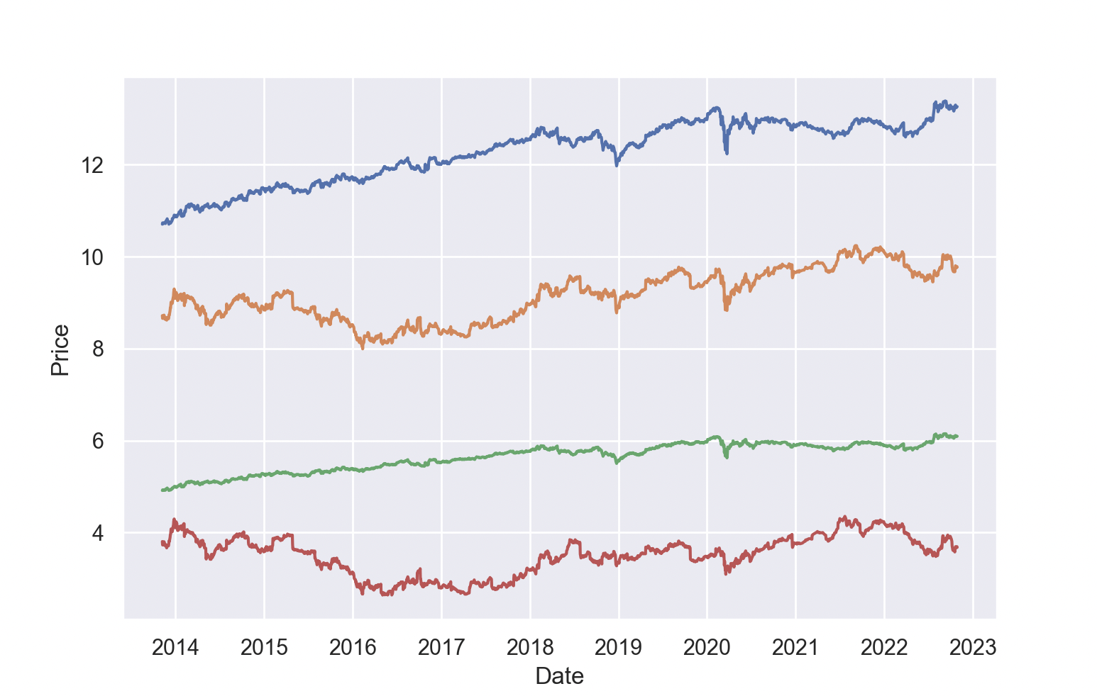
Recall that we didn’t actually buy any MacDonald’s. So, we have—blue, being our “optimal” portfolio, yellow, our balanced portfolio, green, being Lockheed, and red, being Twitter.
Our portfolio works surprisingly well!