cal.com
Last edited: August 8, 2025cal.com is an automating calendar service funded by the VC firm 776.
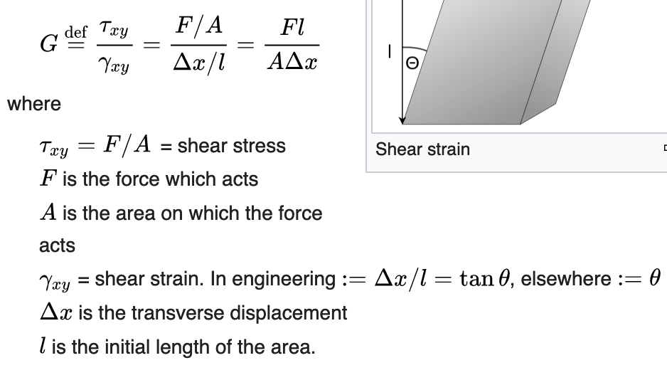
calculating shear's modulus
Last edited: August 8, 2025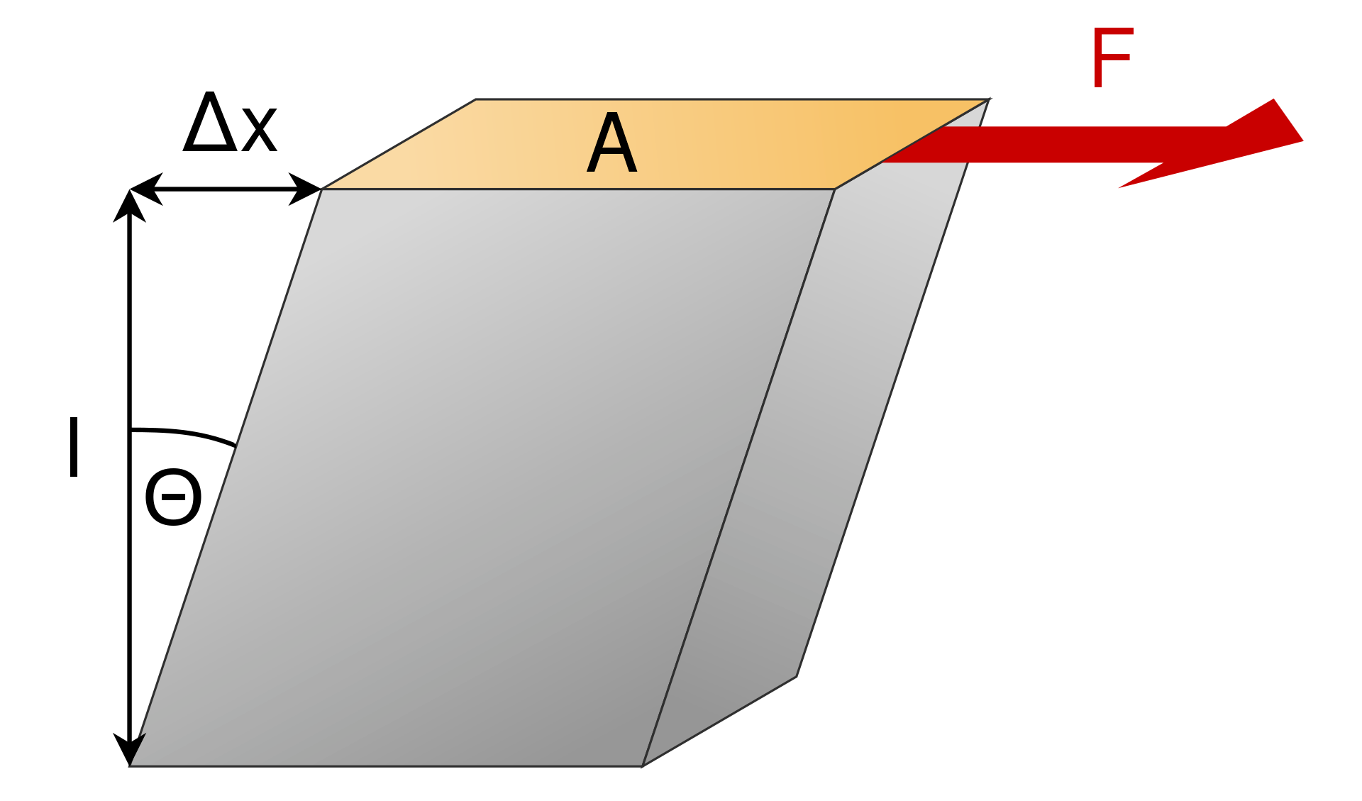
Calibration Plot
Last edited: August 8, 2025call by value
Last edited: August 8, 2025CALP
Last edited: August 8, 2025Contraindicated offline POMDP solver.
- Contrained belief state MDP
- Linear Programming
- belief set generation
- Approximate POMDP with Contrainst
CPOMDPs are Hard
- Can’t do DP with pruning: optimal policies may be stochastic
- Minimax quadratically contained program: computational intractable
- Contained PBVI struggles with contraint satisfaction
CALP Core Idea
Recast CPOMDP as a contrained belief-state MDP.
We replace our state-space with our belief space:
- \(S = B\)
- \(s_0 = b_0\)
You essentially assume here that there is some finite belief space.