iStudio Meeting Notes
Last edited: August 8, 2025| Date | Notes |
|---|---|
| PCP April Checkin | |
| Alivio April Checkin | |
| GreenSwing April Checkin | |
| Pollen April Checkin | |
| Logan’s Team Checkin | |
| Anna’s Team Checkin |
TODO Stack
- Get asthma kids leads for Alivio
- GreenSwing Hiring: Fufilling Orders, MechE
- Conrad money?
- Get Mentors for Pollen => Figma lady
Item Response Theory
Last edited: August 8, 2025If a student has ability \(a\), and a probably is \(d\) difficulty, the probability of a student getting something right:
\begin{equation} \sigma (a-d) \end{equation}
this doesn’t consider SLIPPING at all.
Itô Intergral
Last edited: August 8, 2025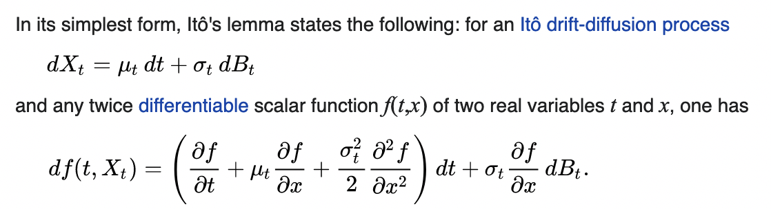
https://en.wikipedia.org/wiki/It%C3%B4%27s_lemma
for integrating Differential Equations with Brownian Motion.